Directive 2005/55/EC of the European Parliament and of the Council (repealed)Dangos y teitl llawn

ANNEX VII EXAMPLE OF CALCULATION PROCEDURE

1. ESC TEST

1.1. Gaseous emissions

The measurement data for the calculation of the individual mode results are shown below. In this example, CO and NO_x are measured on a dry basis, HC on a wet basis. The HC concentration is given in propane equivalent (C3) and has to be multiplied by 3 to result in the C1 equivalent. The calculation procedure is identical for the other modes.

P(kW)	Ta(K)	Ha(g/kg)	GEXH(kg)	GAIRW(kg)	GFUEL(kg)	HC(ppm)	CO(ppm)	NOx(ppm)
82,9	294,8	7,81	563,38	545,29	18,09	6,3	41,2	495

Calculation of the dry to wet correction factor K_W,r (Annex III, Appendix 1, Section 4.2):

and

Calculation of the wet concentrations:

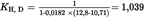
Calculation of the NO_x humidity correction factor K_H,D (Annex III, Appendix 1, Section 4.3):

Calculation of the emission mass flow rates (Annex III, Appendix 1, Section 4.4):

Calculation of the specific emissions (Annex III, Appendix 1, Section 4.5):

The following example calculation is given for CO; the calculation procedure is identical for the other components.

The emission mass flow rates of the individual modes are multiplied by the respective weighting factors, as indicated in Annex III, Appendix 1, Section 2.7.1, and summed up to result in the mean emission mass flow rate over the cycle:

CO	=
	=	30,91 g/h

The engine power of the individual modes is multiplied by the respective weighting factors, as indicated in Annex III, Appendix 1, Section 2.7.1, and summed up to result in the mean cycle power:

	=
	=	60,006 kW

Calculation of the specific NO_x emission of the random point (Annex III, Appendix 1, Section 4.6.1):

Assume the following values have been determined on the random point:

n_Z

=

1 600 min^-1

M_Z

=

495 Nm

NO_{x mass,Z}

=

487,9 g/h (calculated according to the previous formulae)

P(n)_Z

=

83 kW

NO_x,Z

=

487,9/83 = 5,878 g/kWh

Determination of the emission value from the test cycle (Annex III, Appendix 1, Section 4.6.2):

Assume the values of the four enveloping modes on the ESC to be as follows:

nRT	nSU	ER	ES	ET	EU	MR	MS	MT	MU
1 368	1 785	5,943	5,565	5,889	4,973	515	460	681	610

Comparison of the NO_x emission values (Annex III, Appendix 1, Section 4.6.3):

1.2. Particulate emissions

Particulate measurement is based on the principle of sampling the particulates over the complete cycle, but determining the sample and flow rates (M_SAM and G_EDF) during the individual modes. The calculation of G_EDF depends on the system used. In the following examples, a system with CO₂ measurement and carbon balance method and a system with flow measurement are used. When using a full flow dilution system, G_EDF is directly measured by the CVS equipment.

Calculation of G_EDF (Annex III, Appendix 1, Sections 5.2.3 and 5.2.4):

Assume the following measurement data of mode 4. The calculation procedure is identical for the other modes.

GEXH(kg/h)	GFUEL(kg/h)	GDILW(kg/h)	GTOTW(kg/h)	CO2D(%)	CO2A(%)
334,02	10,76	5,4435	6,0	0,657	0,04

(a)

carbon balance method

(b)

flow measurement method

Calculation of the mass flow rate (Annex III, Appendix 1, Section 5.4):

The G_EDFW flow rates of the individual modes are multiplied by the respective weighting factors, as indicated in Annex III, Appendix 1, Section 2.7.1, and summed up to result in the mean G_EDF over the cycle. The total sample rate M_SAM is summed up from the sample rates of the individual modes.

	=
	=	3 604,6 kg/h
	=	0,226 + 0,122 + 0,151 + 0,152 + 0,076 + 0,076 + 0,076 + 0,136 + 0,151 + 0,121 + 0,076 + 0,076 + 0,075
	=	1,515 kg

Assume the particulate mass on the filters to be 2,5 mg, then

Background correction (optional)

Assume one background measurement with the following values. The calculation of the dilution factor DF is identical to Section 3.1 of this Annex and not shown here.

Sum of DF	=
	=	0,923

Calculation of the specific emission (Annex III, Appendix 1, Section 5.5):

	=
	=	60,006 kW

Calculation of the specific weighting factor (Annex III, Appendix 1, Section 5.6):

Assume the values calculated for mode 4 above, then

This value is within the required value of 0,10 ± 0,003.

2. ELR TEST

Since Bessel filtering is a completely new averaging procedure in European exhaust legislation, an explanation of the Bessel filter, an example of the design of a Bessel algorithm, and an example of the calculation of the final smoke value is given below. The constants of the Bessel algorithm only depend on the design of the opacimeter and the sampling rate of the data acquisition system. It is recommended that the opacimeter manufacturer provide the final Bessel filter constants for different sampling rates and that the customer use these constants for designing the Bessel algorithm and for calculating the smoke values.

2.1. General remarks on the Bessel filter

Due to high frequency distortions, the raw opacity signal usually shows a highly scattered trace. To remove these high frequency distortions a Bessel filter is required for the ELR-test. The Bessel filter itself is a recursive, second-order low-pass filter which guarantees the fastest signal rise without overshoot.

Assuming a real time raw exhaust plume in the exhaust tube, each opacimeter shows a delayed and differently measured opacity trace. The delay and the magnitude of the measured opacity trace is primarily dependent on the geometry of the measuring chamber of the opacimeter, including the exhaust sample lines, and on the time needed for processing the signal in the electronics of the opacimeter. The values that characterise these two effects are called the physical and the electrical response time which represent an individual filter for each type of opacimeter.

The goal of applying a Bessel filter is to guarantee a uniform overall filter characteristic of the whole opacimeter system, consisting of:

• physical response time of the opacimeter (t_p),

• electrical response time of the opacimeter (t_e),

• filter response time of the applied Bessel filter (t_F).

The resulting overall response time of the system t_Aver is given by:

and must be equal for all kinds of opacimeters in order to give the same smoke value. Therefore, a Bessel filter has to be created in such a way, that the filter response time (t_F) together with the physical (t_p) and electrical response time (t_e) of the individual opacimeter must result in the required overall response time (t_Aver). Since t_p and t_e are given values for each individual opacimeter, and t_Aver is defined to be 1,0 s in this Directive, t_F can be calculated as follows:

By definition, the filter response time t_F is the rise time of a filtered output signal between 10 % and 90 % on a step input signal. Therefore the cut-off frequency of the Bessel filter has to be iterated in such a way, that the response time of the Bessel filter fits into the required rise time.

In Figure a, the traces of a step input signal and Bessel filtered output signal as well as the response time of the Bessel filter (t_F) are shown.

Designing the final Bessel filter algorithm is a multi step process which requires several iteration cycles. The scheme of the iteration procedure is presented below.

2.2. Calculation of the Bessel algorithm

In this example a Bessel algorithm is designed in several steps according to the above iteration procedure which is based upon Annex III, Appendix 1, Section 6.1.

For the opacimeter and the data acquisition system, the following characteristics are assumed:

• physical response time t_p 0,15 s

• electrical response time t_e 0,05 s

• overall response time t_Aver 1,00 s (by definition in this Directive)

• sampling rate 150 Hz

Step 1 Required Bessel filter response time t_F:

Step 2 Estimation of cut-off frequency and calculation of Bessel constants E, K for first iteration:

f_c

=

Δt

=

1/150 = 0,006667 s

Ω

=

E

=

K

=

This gives the Bessel algorithm:

where S_i represents the values of the step input signal (either ‘0’ or ‘1’) and Y_i represents the filtered values of the output signal.

Step 3 Application of Bessel filter on step input:

The Bessel filter response time t_F is defined as the rise time of the filtered output signal between 10 % and 90 % on a step input signal. For determining the times of 10 % (t₁₀) and 90 % (t₉₀) of the output signal, a Bessel filter has to be applied to a step input using the above values of f_c, E and K.

The index numbers, the time and the values of a step input signal and the resulting values of the filtered output signal for the first and the second iteration are shown in Table B. The points adjacent to t₁₀ and t₉₀ are marked in bold numbers.

In Table B, first iteration, the 10 % value occurs between index number 30 and 31 and the 90 % value occurs between index number 191 and 192. For the calculation of t_F,iter the exact t₁₀ and t₉₀ values are determined by linear interpolation between the adjacent measuring points, as follows:

where out_upper and out_lower, respectively, are the adjacent points of the Bessel filtered output signal, and t_lower is the time of the adjacent time point, as indicated in Table B.

Step 4 Filter response time of first iteration cycle:

Step 5 Deviation between required and obtained filter response time of first iteration cycle:

Step 6 Checking the iteration criteria:

|Δ| ≤ 0,01 is required. Since 0,081641 > 0,01, the iteration criteria is not met and a further iteration cycle has to be started. For this iteration cycle, a new cut-off frequency is calculated from f_c and Δ as follows:

This new cut-off frequency is used in the second iteration cycle, starting at step 2 again. The iteration has to be repeated until the iteration criteria is met. The resulting values of the first and second iteration are summarised in Table A.

Table A

Values of the first and second iteration

Parameter		1. Iteration	2. Iteration
fc	(Hz)	0,318152	0,344126
E	(-)	7,07948 E-5	8,272777 E-5
K	(-)	0,970783	0,96841
t10	(s)	0,200945	0,185523
t90	(s)	1,276147	1,179562
tF,iter	(s)	1,075202	0,994039
Δ	(-)	0,081641	0,006657
fc,new	(Hz)	0,344126	0,346417

Step 7 Final Bessel algorithm:

As soon as the iteration criteria has been met, the final Bessel filter constants and the final Bessel algorithm are calculated according to step 2. In this example, the iteration criteria has been met after the second iteration (Δ = 0,006657 ≤ 0,01). The final algorithm is then used for determining the averaged smoke values (see next Section 2.3).

Table B

Values of step input signal and Bessel filtered output signal for the first and second iteration cycle

Index i[-]	Time[s]	Step input signal Si[-]	Filtered output signal Yi[-]
			1. Iteration	2. Iteration
- 2	- 0,013333	0	0,0	0,0
- 1	- 0,006667	0	0,0	0,0
0	0,0	1	0,000071	0,000083
1	0,006667	1	0,000352	0,000411
2	0,013333	1	0,000908	0,00106
3	0,02	1	0,001731	0,002019
4	0,026667	1	0,002813	0,003278
5	0,033333	1	0,004145	0,004828
~	~	~	~	~
24	0,16	1	0,067877	0,077876
25	0,166667	1	0,072816	0,083476
26	0,173333	1	0,077874	0,089205
27	0,18	1	0,083047	0,095056
28	0,186667	1	0,088331	0,101024
29	0,193333	1	0,093719	0,107102
30	0,2	1	0,099208	0,113286
31	0,206667	1	0,104794	0,11957
32	0,213333	1	0,110471	0,125949
33	0,22	1	0,116236	0,132418
34	0,226667	1	0,122085	0,138972
35	0,233333	1	0,128013	0,145605
36	0,24	1	0,134016	0,152314
37	0,246667	1	0,140091	0,159094
~	~	~	~	~
175	1,166667	1	0,862416	0,895701
176	1,173333	1	0,864968	0,897941
177	1,18	1	0,867484	0,900145
178	1,186667	1	0,869964	0,902312
179	1,193333	1	0,87241	0,904445
180	1,2	1	0,874821	0,906542
181	1,206667	1	0,877197	0,908605
182	1,213333	1	0,87954	0,910633
183	1,22	1	0,881849	0,912628
184	1,226667	1	0,884125	0,914589
185	1,233333	1	0,886367	0,916517
186	1,24	1	0,888577	0,918412
187	1,246667	1	0,890755	0,920276
188	1,253333	1	0,8929	0,922107
189	1,26	1	0,895014	0,923907
190	1,266667	1	0,897096	0,925676
191	1,273333	1	0,899147	0,927414
192	1,28	1	0,901168	0,929121
193	1,286667	1	0,903158	0,930799
194	1,293333	1	0,905117	0,932448
195	1,3	1	0,907047	0,934067
~	~	~	~	~

2.3. Calculation of the smoke values

In the scheme below the general procedure of determining the final smoke value is presented.

In Figure b, the traces of the measured raw opacity signal, and of the unfiltered and filtered light absorption coefficients (k-value) of the first load step of an ELR-Test are shown, and the maximum value Y_max1,A (peak) of the filtered k trace is indicated. Correspondingly, Table C contains the numerical values of index i, time (sampling rate of 150 Hz), raw opacity, unfiltered k and filtered k. Filtering was conducted using the constants of the Bessel algorithm designed in Section 2.2 of this Annex. Due to the large amount of data, only those sections of the smoke trace around the beginning and the peak are tabled.

The peak value (i = 272) is calculated assuming the following data of Table C. All other individual smoke values are calculated in the same way. For starting the algorithm, S_-1, S_-2, Y_-1 and Y_-2 are set to zero.

LA (m)	0,43
Index i	272
N ( %)	16,783
S271 (m-1)	0,427392
S270 (m-1)	0,427532
Y271 (m-1)	0,542383
Y270 (m-1)	0,542337

Calculation of the k-value (Annex III, Appendix 1, Section 6.3.1):

This value corresponds to S₂₇₂ in the following equation.

Calculation of Bessel averaged smoke (Annex III, Appendix 1, Section 6.3.2):

In the following equation, the Bessel constants of the previous Section 2.2 are used. The actual unfiltered k-value, as calculated above, corresponds to S₂₇₂ (S_i). S₂₇₁ (S_i-1) and S₂₇₀ (S_i-2) are the two preceding unfiltered k-values, Y₂₇₁ (Y_i-1) and Y₂₇₀ (Y_i-2) are the two preceding filtered k-values.

	=
	=

This value corresponds to Y_max1,A in the following equation.

Calculation of the final smoke value (Annex III, Appendix 1, Section 6.3.3):

From each smoke trace, the maximum filtered k-value is taken for the further calculation.

Assume the following values

Speed	Ymax (m-1)
	Cycle 1	Cycle 2	Cycle 3
A	0,5424	0,5435	0,5587
B	0,5596	0,54	0,5389
C	0,4912	0,5207	0,5177

Cycle validation (Annex III, Appendix 1, Section 3.4)

Before calculating SV, the cycle must be validated by calculating the relative standard deviations of the smoke of the three cycles for each speed.

Speed	Mean SV(m-1)	Absolute standard deviation(m-1)	Relative standard deviation(%)
A	0,5482	0,0091	1,7
B	0,5462	0,0116	2,1
C	0,5099	0,0162	3,2

In this example, the validation criteria of 15 % are met for each speed.

Table C

Values of opacity N, unfiltered and filtered k-value at beginning of load step

Index i[-]	Time[s]	Opacity N[%]	Unfiltered k-value[m-1]	Filtered k-value[m-1]
- 2	0,0	0,0	0,0	0,0
- 1	0,0	0,0	0,0	0,0
0	0,0	0,0	0,0	0,0
1	0,006667	0,02	0,000465	0,0
2	0,013333	0,02	0,000465	0,0
3	0,02	0,02	0,000465	0,0
4	0,026667	0,02	0,000465	0,000001
5	0,033333	0,02	0,000465	0,000002
6	0,04	0,02	0,000465	0,000002
7	0,046667	0,02	0,000465	0,000003
8	0,053333	0,02	0,000465	0,000004
9	0,06	0,02	0,000465	0,000005
10	0,066667	0,02	0,000465	0,000006
11	0,073333	0,02	0,000465	0,000008
12	0,08	0,02	0,000465	0,000009
13	0,086667	0,02	0,000465	0,000011
14	0,093333	0,02	0,000465	0,000012
15	0,1	0,192	0,004469	0,000014
16	0,106667	0,212	0,004935	0,000018
17	0,113333	0,212	0,004935	0,000022
18	0,12	0,212	0,004935	0,000028
19	0,126667	0,343	0,00799	0,000036
20	0,133333	0,566	0,0132	0,000047
21	0,14	0,889	0,020767	0,000061
22	0,146667	0,929	0,021706	0,000082
23	0,153333	0,929	0,021706	0,000109
24	0,16	1,263	0,029559	0,000143
25	0,166667	1,455	0,034086	0,000185
26	0,173333	1,697	0,039804	0,000237
27	0,18	2,03	0,047695	0,000301
28	0,186667	2,081	0,048906	0,000378
29	0,193333	2,081	0,048906	0,000469
30	0,2	2,424	0,057067	0,000573
31	0,206667	2,475	0,058282	0,000693
32	0,213333	2,475	0,058282	0,000827
33	0,22	2,808	0,066237	0,000977
34	0,226667	3,01	0,071075	0,001144
35	0,233333	3,253	0,076909	0,001328
36	0,24	3,606	0,08541	0,001533
37	0,246667	3,96	0,093966	0,001758
38	0,253333	4,455	0,105983	0,002007
39	0,26	4,818	0,114836	0,002283
40	0,266667	5,02	0,119776	0,002587

Values of opacity N, unfiltered and filtered k-value around Y_max1,A (≡ peak value, indicated in bold number)

Index i[-]	Time[s]	Opacity N[%]	Unfiltered k-value[m-1]	Filtered k-value[m-1]
259	1,726667	17,182	0,438429	0,538856
260	1,733333	16,949	0,431896	0,539423
261	1,74	16,788	0,427392	0,539936
262	1,746667	16,798	0,427671	0,540396
263	1,753333	16,788	0,427392	0,540805
264	1,76	16,798	0,427671	0,541163
265	1,766667	16,798	0,427671	0,541473
266	1,773333	16,788	0,427392	0,541735
267	1,78	16,788	0,427392	0,541951
268	1,786667	16,798	0,427671	0,542123
269	1,793333	16,798	0,427671	0,542251
270	1,8	16,793	0,427532	0,542337
271	1,806667	16,788	0,427392	0,542383
272	1,813333	16,783	0,427252	0,542389
273	1,82	16,78	0,427168	0,542357
274	1,826667	16,798	0,427671	0,542288
275	1,833333	16,778	0,427112	0,542183
276	1,84	16,808	0,427951	0,542043
277	1,846667	16,768	0,426833	0,54187
278	1,853333	16,01	0,40575	0,541662
279	1,86	16,01	0,40575	0,541418
280	1,866667	16,0	0,405473	0,541136
281	1,873333	16,01	0,40575	0,540819
282	1,88	16,0	0,405473	0,540466
283	1,886667	16,01	0,40575	0,54008
284	1,893333	16,394	0,416406	0,539663
285	1,9	16,394	0,416406	0,539216
286	1,906667	16,404	0,416685	0,538744
287	1,913333	16,394	0,416406	0,538245
288	1,92	16,394	0,416406	0,537722
289	1,926667	16,384	0,416128	0,537175
290	1,933333	16,01	0,40575	0,536604
291	1,94	16,01	0,40575	0,536009
292	1,946667	16,0	0,405473	0,535389
293	1,953333	16,01	0,40575	0,534745
294	1,96	16,212	0,411349	0,534079
295	1,966667	16,394	0,416406	0,533394
296	1,973333	16,394	0,416406	0,532691
297	1,98	16,192	0,410794	0,531971
298	1,986667	16,0	0,405473	0,531233
299	1,993333	16,0	0,405473	0,530477
300	2,0	16,0	0,405473	0,529704

3. ETC TEST

3.1. Gaseous emissions (diesel engine)

Assume the following test results for a PDP-CVS system

V0 (m3/rev)	0,1776
Np (rev)	23 073
pB (kPa)	98,0
p1 (kPa)	2,3
T (K)	322,5
Ha (g/kg)	12,8
NOx conce (ppm)	53,7
NOx concd (ppm)	0,4
COconce (ppm)	38,9
COconcd (ppm)	1,0
HCconce (ppm)	9,0
HCconcd (ppm)	3,02
CO2,conce (%)	0,723
Wact (kWh)	62,72

Calculation of the diluted exhaust gas flow (Annex III, Appendix 2, Section 4.1):

Calculation of the NO_x correction factor (Annex III, Appendix 2, Section 4.2):

Calculation of the background corrected concentrations (Annex III, Appendix 2, Section 4.3.1.1):

Assuming a diesel fuel of the composition C₁H_1,8

Calculation of the emissions mass flow (Annex III, Appendix 2, Section 4.3.1):

Calculation of the specific emissions (Annex III, Appendix 2, Section 4.4):

3.2. Particulate emissions (diesel engine)

Assume the following test results for a PDP-CVS system with double dilution

MTOTW (kg)	4 237,2
Mf,p (mg)	3,03
Mf,b (mg)	0,044
MTOT (kg)	2,159
MSEC (kg)	0,909
Md (mg)	0,341
MDIL (kg)	1,245
DF	18,69
Wact (kWh)	62,72

Calculation of the mass emission (Annex III, Appendix 2, Section 5.1):

Calculation of the background corrected mass emission (Annex III, Appendix 2, Section 5.1):

Calculation of the specific emission (Annex III, Appendix 2, Section 5.2):

3.3. Gaseous emissions (CNG engine)

Assume the following test results for a PDP-CVS system with double dilution

MTOTW (kg)	4 237,2
Ha (g/kg)	12,8
NOx conce (ppm)	17,2
NOx concd (ppm)	0,4
COconce (ppm)	44,3
COconcd (ppm)	1,0
HCconce (ppm)	27,0
HCconcd (ppm)	3,02
CH4 conce (ppm)	18,0
CH4 concd (ppm)	1,7
CO2,conce ( %)	0,723
Wact (kWh)	62,72

Calculation of the NO_x, correction factor (Annex III, Appendix 2, Section 4.2):

Calculation of the NMHC concentration (Annex III, Appendix 2, Section 4.3.1):

(a)

GC method

(b)

NMC method

Assuming a methane efficiency of 0,04 and an ethane efficiency of 0,98 (see Annex III, Appendix 5, Section 1.8.4)

Calculation of the background corrected concentrations (Annex III, Appendix 2, Section 4.3.1.1):

Assuming a G₂₀ reference fuel (100 % methane) of the composition C₁H₄:

For NMHC, the background concentration is the difference between HC_concd and CH_4concd

Calculation of the emissions mass flow (Annex III, Appendix 2, Section 4.3.1):

Calculation of the specific emissions (Annex III, Appendix 2, Section 4.4):

4. λ-SHIFT FACTOR (S_λ)

4.1. Calculation of the λ-shift factor (S_λ)(1)

where:

S_λ

=

λ-shift factor;

inert %

=

% by volume of inert gases in the fuel (i.e. N₂, CO₂, He, etc.);

O₂ ^*

=

% by volume of original oxygen in the fuel;

n and m

=

refer to average C_nH_m representing the fuel hydrocarbons, i.e:

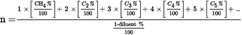
where:

CH₄

=

% by volume of methane in the fuel;

C₂

=

% by volume of all C₂ hydrocarbons (e.g. C₂H₆, C₂H₄, etc.) in the fuel;

C₃

=

% by volume of all C₃ hydrocarbons (e.g. C₃H₈, C₃H₆, etc.) in the fuel;

C₄

=

% by volume of all C₄ hydrocarbons (e.g. C₄H₁₀, C₄H₈, etc.) in the fuel

C₅

=

% by volume of all C₅ hydrocarbons (e.g. C₅H₁₂, C₅H₁₀, etc.) in the fuel;

diluent

=

% by volume of dilution gases in the fuel (i.e. O₂ ^*, N₂, CO₂, He etc.).

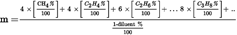
4.2. Examples for the calculation of the λ-shift factor S_λ

Example 1: G₂₅: CH₄ = 86 %, N₂ = 14 % (by volume)

Example 2: GR: CH₄ = 87 %, C₂H₆ = 13 % (by vol)

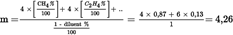
Example 3: USA: CH₄ = 89 %, C₂H₆ = 4,5 %, C₃H₈ = 2,3 %, C₆H₁₄ = 0,2 %, O₂ = 0,6 %, N₂ = 4 %

(1)

Stoichiometric Air/Fuel ratios of automotive fuels - SAE J1829, June 1987. John B. Heywood, Internal combustion engine fundamentals, McGraw-Hill, 1988, Chapter 3.4 ‘Combustion stoichiometry’ (pp. 68 to 72).