- Y Diweddaraf sydd Ar Gael (Diwygiedig)
- Pwynt Penodol mewn Amser (31/12/2020)
- Gwreiddiol (Fel y’i mabwysiadwyd gan yr UE)
Commission Directive (EU) 2015/996Dangos y teitl llawn
Commission Directive (EU) 2015/996 of 19 May 2015 establishing common noise assessment methods according to Directive 2002/49/EC of the European Parliament and of the Council (Text with EEA relevance)
You are here:
- Cyfarwyddebau yn deillio o’r UE
- 2015 No. 996
- ANNEX
- Division ASSESSMENT METHODS FOR THE NOISE INDICATORS

Pa Fersiwn
Nodweddion Uwch
- Dangos Graddfa Ddaearyddol(e.e. Lloegr, Cymru, Yr Alban aca Gogledd Iwerddon)
- Dangos Llinell Amser Newidiadau
Rhagor o Adnoddau
Legislation originating from the EU
When the UK left the EU, legislation.gov.uk published EU legislation that had been published by the EU up to IP completion day (31 December 2020 11.00 p.m.). On legislation.gov.uk, these items of legislation are kept up-to-date with any amendments made by the UK since then.


Mae hon yn eitem o ddeddfwriaeth sy’n deillio o’r UE
Mae unrhyw newidiadau sydd wedi cael eu gwneud yn barod gan y tîm yn ymddangos yn y cynnwys a chyfeirir atynt gydag anodiadau.Ar ôl y diwrnod ymadael bydd tair fersiwn o’r ddeddfwriaeth yma i’w gwirio at ddibenion gwahanol. Y fersiwn legislation.gov.uk yw’r fersiwn sy’n weithredol yn y Deyrnas Unedig. Y Fersiwn UE sydd ar EUR-lex ar hyn o bryd yw’r fersiwn sy’n weithredol yn yr UE h.y. efallai y bydd arnoch angen y fersiwn hon os byddwch yn gweithredu busnes yn yr UE. EUR-Lex Y fersiwn yn yr archif ar y we yw’r fersiwn swyddogol o’r ddeddfwriaeth fel yr oedd ar y diwrnod ymadael cyn cael ei chyhoeddi ar legislation.gov.uk ac unrhyw newidiadau ac effeithiau a weithredwyd yn y Deyrnas Unedig wedyn. Mae’r archif ar y we hefyd yn cynnwys cyfraith achos a ffurfiau mewn ieithoedd eraill o EUR-Lex. The EU Exit Web Archive legislation_originated_from_EU_p3
Changes over time for: Division ASSESSMENT METHODS FOR THE NOISE INDICATORS
Alternative versions:
Status:
EU Directives are published on this site to aid cross referencing from UK legislation. Since IP completion day (31 December 2020 11.00 p.m.) no amendments have been applied to this version.
ASSESSMENT METHODS FOR THE NOISE INDICATORS (Referred to in Article 6 of Directive 2002/49/EC)U.K.
1.INTRODUCTIONU.K.
The values of Lden and Lnight shall be determined at the assessment positions by computation, according to the method set out in Chapter 2 and the data described in Chapter 3. Measurements may be performed according to Chapter 4.
2.COMMON NOISE ASSESSMENT METHODSU.K.
2.1. General provisions — Road traffic, railway and industrial noise U.K.
2.1.1. Indicators, frequency range and band definitions U.K.
Noise calculations shall be defined in the frequency range from 63 Hz to 8 kHz. Frequency band results shall be provided at the corresponding frequency interval.
Calculations are performed in octave bands for road traffic, railway traffic and industrial noise, except for the railway noise source sound power, that uses third octave bands. For road traffic, railway traffic and industrial noise, based on these octave band results, the A-weighted long term average sound pressure level for the day, evening and night period, as defined in Annex I and referred to in Art. 5 of Directive 2002/49/EC, is computed by summation over all frequencies:

where
Ai denotes the A-weighting correction according to IEC 61672-1
i = frequency band index
and T is the time period corresponding to day, evening or night.
Noise parameters:
| Lp | Instantaneous sound pressure level | [dB] (re. 2 10–5 Pa) |
| LAeq,LT | Global long-term sound level LAeq due to all sources and image sources at point R | [dB] (re. 2 10–5 Pa) |
| LW | ‘In situ’ sound power level of a point source (moving or steady) | [dB] (re. 10–12 W) |
| LW,i,dir | Directional ‘in situ’ sound power level for the i-th frequency band | [dB] (re. 10–12 W) |
| LW′ | Average ‘in situ’ sound power level per metre of source line | [dB/m] (re. 10–12 W) |
Other physical parameters:
| p | r.m.s. of the instantaneous sound pressure | [Pa] |
| p 0 | Reference sound pressure = 2 10–5 Pa | [Pa] |
| W 0 | Reference sound power = 10–12 W | [watt] |
2.1.2. Quality framework U.K.
Accuracy of input values U.K.
All input values affecting the emission level of a source shall be determined with at least the accuracy corresponding to an uncertainty of ± 2dB(A) in the emission level of the source (leaving all other parameters unchanged).
Use of default values U.K.
In the application of the method, the input data shall reflect the actual usage. In general there shall be no reliance on default input values or assumptions. Default input values and assumptions are accepted if the collection of real data is associated with disproportionately high costs.
Quality of the software used for the calculations U.K.
Software used to perform the calculations shall prove compliance with the methods herewith described by means of certification of results against test cases.
2.2. Road traffic noise U.K.
2.2.1. Source description U.K.
Classification of vehicles U.K.
The road traffic noise source shall be determined by combining the noise emission of each individual vehicle forming the traffic flow. These vehicles are grouped into five separate categories with regard to their characteristics of noise emission:
Category 1
:
Light motor vehicles
Category 2
:
Medium heavy vehicles
Category 3
:
Heavy vehicles
Category 4
:
Powered two-wheelers
Category 5
:
Open category
In the case of powered two-wheelers, two separate subclasses are defined for mopeds and more powerful motorcycles, since they operate in very different driving modes and their numbers usually vary widely.
The first four categories shall be used, and the fifth category is optional. It is foreseen for new vehicles that may be developed in the future and may be sufficiently different in their noise emission to require an additional category to be defined. This category could cover, for example, electric or hybrid vehicles or any vehicle developed in the future substantially different from those in categories 1 to 4.
The details of the different vehicle classes are given in Table [2.2.a].
Table [2.2.a]
Vehicle classes
| a Directive 2007/46/EC of the European Parliament and of the Council of 5 September 2007 establishing a framework for the approval of motor vehicles and their trailers, and of systems, components and separate technical units intended for such vehicles (OJ L 263, 9.10.2007, p. 1). | ||||
| b Sport Utility Vehicles. | ||||
| c Multi-Purpose Vehicles. | ||||
| Category | Name | Description | Vehicle category in ECWhole Vehicle Type Approvala | |
|---|---|---|---|---|
| 1 | Light motor vehicles | Passenger cars, delivery vans ≤ 3,5 tons, SUVsb, MPVsc including trailers and caravans | M1 and N1 | |
| 2 | Medium heavy vehicles | Medium heavy vehicles, delivery vans > 3,5 tons, buses, motorhomes, etc. with two axles and twin tyre mounting on rear axle | M2, M3 and N2, N3 | |
| 3 | Heavy vehicles | Heavy duty vehicles, touring cars, buses, with three or more axles | M2 and N2 with trailer, M3 and N3 | |
| 4 | Powered two-wheelers | 4a | Two-, Three- and Four-wheel Mopeds | L1, L2, L6 |
| 4b | Motorcycles with and without sidecars, Tricycles and Quadricycles | L3, L4, L5, L7 | ||
| 5 | Open category | To be defined according to future needs | N/A | |
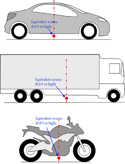
Number and position of equivalent sound sources U.K.
In this method, each vehicle (category 1, 2, 3, 4 and 5) is represented by one single point source radiating uniformly into the 2-π half space above the ground. The first reflection on the road surface is treated implicitly. As depicted in Figure [2.2.a], this point source is placed 0,05 m above the road surface.
Figure [2.2.a]
Location of equivalent point source on light vehicles (category 1), heavy vehicles (categories 2 and 3) and two-wheelers (category 4)
The traffic flow is represented by a source line. In the modelling of a road with multiple lanes, each lane should ideally be represented by a source line placed in the centre of each lane. However, it is also acceptable to model one source line in the middle of a two way road or one source line per carriageway in the outer lane of multi-lane roads.
Sound power emission U.K.
General considerations U.K.
The sound power of the source is defined in the ‘semi-free field’, thus the sound power includes the effect of the reflection of the ground immediately under the modelled source where there are no disturbing objects in its immediate surroundings except for the reflection on the road surface not immediately under the modelled source.
Traffic flow U.K.
The noise emission of a traffic flow is represented by a source line characterised by its directional sound power per metre per frequency. This corresponds to the sum of the sound emission of the individual vehicles in the traffic flow, taking into account the time spent by the vehicles in the road section considered. The implementation of the individual vehicle in the flow requires the application of a traffic flow model.
If a steady traffic flow of Qm vehicles of category m per hour is assumed, with an average speed vm (in km/h), the directional sound power per metre in frequency band i of the source line LW′, eq,line,i,m is defined by:

where LW,i,m is the directional sound power of a single vehicle. LW′,m is expressed in dB (re. 10–12 W/m). These sound power levels are calculated for each octave band i from 125 Hz to 4 kHz.
Traffic flow data Qm shall be expressed as yearly average per hour, per time period (day-evening-night), per vehicle class and per source line. For all categories, input traffic flow data derived from traffic counting or from traffic models shall be used.
The speed vm is a representative speed per vehicle category: in most cases the lower of the maximum legal speed for the section of road and the maximum legal speed for the vehicle category. If local measurement data is unavailable the maximum legal speed for the vehicle category shall be used.
Individual vehicle U.K.
In the traffic flow, all vehicles of category m are assumed to drive at the same speed, i.e. vm , the average speed of the flow of vehicles of the category.
A road vehicle is modelled by a set of mathematical equations representing the two main noise sources:
1.
Rolling noise due to the tyre/road interaction;
2.
Propulsion noise produced by the driveline (engine, exhaust, etc.) of the vehicle.
Aerodynamic noise is incorporated in the rolling noise source.
For light, medium and heavy motor vehicles (categories 1, 2 and 3), the total sound power corresponds to the energetic sum of the rolling and the propulsion noise. Thus, the total sound power level of the source lines m = 1, 2 or 3 is defined by:

where LWR,i,m is the sound power level for rolling noise and LWP,i,m is the sound power level for propulsion noise. This is valid on all speed ranges. For speeds less than 20 km/h it shall have the same sound power level as defined by the formula for vm = 20 km/h.
For two-wheelers (category 4), only propulsion noise is considered for the source:
| LW,i,m = 4 (vm = 4 ) = LWP,i,m = 4 (vm = 4 ) | (2.2.3) |
This is valid on all speed ranges. For speeds less than 20 km/h it shall have the same sound power level as defined by the formula for vm = 20 km/h.
2.2.2. Reference conditions U.K.
The source equations and coefficients are valid for the following reference conditions:
a constant vehicle speed
a flat road
an air temperature τref = 20 °C
a virtual reference road surface, consisting of an average of dense asphalt concrete 0/11 and stone mastic asphalt 0/11, between 2 and 7 years old and in a representative maintenance condition
a dry road surface
no studded tyres.
2.2.3. Rolling noise U.K.
General equation U.K.
The rolling noise sound power level in the frequency band i for a vehicle of class m = 1,2 or 3 is defined as:

The coefficients AR,i,m and BR,i,m are given in octave bands for each vehicle category and for a reference speed vref = 70 km/h. ΔLWR,i,m corresponds to the sum of the correction coefficients to be applied to the rolling noise emission for specific road or vehicle conditions deviating from the reference conditions:
| ΔLWR,i,m = ΔLWR,road,i,m + ΔLstuddedtyres,i,m + ΔLWR,acc,i,m + ΔLW,temp | (2.2.5) |
ΔLWR,road,i,m accounts for the effect on rolling noise of a road surface with acoustic properties different from those of the virtual reference surface as defined in Chapter 2.2.2. It includes both the effect on propagation and on generation.
ΔLstudded tyres,i,m is a correction coefficient accounting for the higher rolling noise of light vehicles equipped with studded tyres.
ΔLWR,acc,i,m accounts for the effect on rolling noise of a crossing with traffic lights or a roundabout. It integrates the effect on noise of the speed variation.
ΔLW,temp is a correction term for an average temperature τ different from the reference temperature τref = 20 °C.
Correction for studded tyres U.K.
In situations where a significant number of light vehicles in the traffic flow use studded tyres during several months every year, the induced effect on rolling noise shall be taken into account. For each vehicle of category m = 1 equipped with studded tyres, a speed-dependent increase in rolling noise emission is evaluated by:
| Δstud,i (v) = | ai + bi × lg(50/70) for v < 50 km/h | (2.2.6) |
| ai + bi × lg(v/70) for 50 ≤ v ≤ 90 km/h | ||
| ai + bi × lg(90/70) for v > 90 km/h |
where coefficients ai and bi are given for each octave band.
The increase in rolling noise emission shall only be attributed according to the proportion of light vehicles with studded tyres and during a limited period Ts (in months) over the year. If Qstud,ratio is the average ratio of the total volume of light vehicles per hour equipped with studded tyres during the period Ts (in months), then the yearly average proportion of vehicles equipped with studded tyres ps is expressed by:

The resulting correction to be applied to the rolling sound power emission due to the use of studded tyres for vehicles of category m = 1 in frequency band i shall be:

For vehicles of all other categories no correction shall be applied:
| ΔLstuddedtyres,i,m ≠ 1 = 0 | (2.2.9) |
Effect of air temperature on rolling noise correction U.K.
The air temperature affects rolling noise emission; the rolling sound power level decreases when the air temperature increases. This effect is introduced in the road surface correction. Road surface corrections are usually evaluated at an air temperature of τref = 20 °C. In the case of a different yearly average air temperature °C, the road surface noise shall be corrected by:
| ΔLW,temp,m (τ) = Km × (τref – τ) | (2.2.10) |
The correction term is positive (i.e. noise increases) for temperatures lower than 20 °C and negative (i.e. noise decreases) for higher temperatures. The coefficient K depends on the road surface and the tyre characteristics and in general exhibits some frequency dependence. A generic coefficient Km = 1 = 0,08 dB/°C for light vehicles (category 1) and Km = 2 = Km = 3 = 0,04 dB/°C for heavy vehicles (categories 2 and 3) shall be applied for all road surfaces. The correction coefficient shall be applied equally on all octave bands from 63 to 8 000 Hz.
2.2.4. Propulsion noise U.K.
General equation U.K.
The propulsion noise emission includes all contributions from engine, exhaust, gears, air intake, etc. The propulsion noise sound power level in the frequency band i for a vehicle of class m is defined as:

The coefficients AP,i,m and BP,i,m are given in octave bands for each vehicle category and for a reference speed vref = 70 km/h.
ΔLWP,i,m corresponds to the sum of the correction coefficients to be applied to the propulsion noise emission for specific driving conditions or regional conditions deviating from the reference conditions:
| ΔLWP,i,m = ΔLWP,road,i,m + ΔLWP,grad,i,m + ΔLWP,acc,i,m | (2.2.12) |
ΔLWP,road,i,m accounts for the effect of the road surface on the propulsion noise via absorption. The calculation shall be performed according to Chapter 2.2.6.
ΔLWP,acc,i,m and ΔLWP,grad,i,m account for the effect of road gradients and of vehicle acceleration and deceleration at intersections. They shall be calculated according to Chapters 2.2.4 and 2.2.5 respectively.
Effect of road gradients U.K.
The road gradient has two effects on the noise emission of the vehicle: first, it affects the vehicle speed and thus the rolling and propulsion noise emission of the vehicle; second, it affects both the engine load and the engine speed via the choice of gear and thus the propulsion noise emission of the vehicle. Only the effect on the propulsion noise is considered in this section, where a steady speed is assumed.
The effect of the road gradient on the propulsion noise is taken into account by a correction term ΔLWP,grad,m which is a function of the slope s (in %), the vehicle speed vm (in km/h) and the vehicle class m. In the case of a bi-directional traffic flow, it is necessary to split the flow into two components and correct half for uphill and half for downhill. The correction term is attributed to all octave bands equally:
For m = 1
For m = 2
For m = 3
For m = 4
ΔLWP,grad,i,m = 4 = 0 (2.2.16)


The correction ΔLWP,grad,m implicitly includes the effect of slope on speed.
2.2.5. Effect of the acceleration and deceleration of vehicles U.K.
Before and after crossings with traffic lights and roundabouts a correction shall be applied for the effect of acceleration and deceleration as described below.
The correction terms for rolling noise, ΔLWR,acc,m,k , and for propulsion noise, ΔLWP,acc,m,k , are linear functions of the distance x (in m) of the point source to the nearest intersection of the respective source line with another source line. They are attributed to all octave bands equally:
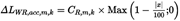

The coefficients CR,m,k and CP,m,k depend on the kind of junction k (k = 1 for a crossing with traffic lights; k = 2 for a roundabout) and are given for each vehicle category. The correction includes the effect of change in speed when approaching or moving away from a crossing or a roundabout.
Note that at a distance |x| ≥ 100 m, ΔLWR,acc,m,k = ΔLWP,acc,m,k = 0.
2.2.6. Effect of the type of road surface U.K.
General principles U.K.
For road surfaces with acoustic properties different from those of the reference surface, a spectral correction term for both rolling noise and propulsion noise shall be applied.
The road surface correction term for the rolling noise emission is given by:

where
αi,m is the spectral correction in dB at reference speed vref for category m (1, 2 or 3) and spectral band i.
βm is the speed effect on the rolling noise reduction for category m (1, 2 or 3) and is identical for all frequency bands.
The road surface correction term for the propulsion noise emission is given by:
| ΔLWP,road,i,m = min{αi,m ;0} | (2.2.20) |
Absorbing surfaces decrease the propulsion noise, while non-absorbing surfaces do not increase it.
Age effect on road surface noise properties U.K.
The noise characteristics of road surfaces vary with age and the level of maintenance, with a tendency to become louder over time. In this method the road surface parameters are derived to be representative for the acoustic performance of the road surface type averaged over its representative lifetime and assuming proper maintenance.
2.3. Railway noise U.K.
2.3.1. Source description U.K.
Classification of vehicles U.K.
Definition of vehicle and train U.K.
For the purposes of this noise calculation method, a vehicle is defined as any single railway sub-unit of a train (typically a locomotive, a self-propelled coach, a hauled coach or a freight wagon) that can be moved independently and can be detached from the rest of the train. Some specific circumstances may occur for sub-units of a train that are a part of a non-detachable set, e.g. share one bogie between them. For the purpose of this calculation method, all these sub-units are grouped into a single vehicle.
For the purpose of this calculation method, a train consists of a series of coupled vehicles.
Table [2.3.a] defines a common language to describe the vehicle types included in the source database. It presents the relevant descriptors to be used to classify the vehicles in full. These descriptors correspond to properties of the vehicle, which affect the acoustic directional sound power per metre length of the equivalent source line modelled.
The number of vehicles for each type shall be determined on each of the track sections for each of the time periods to be used in the noise calculation. It shall be expressed as an average number of vehicles per hour, which is obtained by dividing the total number of vehicles travelling in a given time period by the duration in hours of this time period (e.g. 24 vehicles in 4 hours means 6 vehicles per hour). All vehicle types travelling on each track section shall be used.
Table [2.3.a]
Classification and descriptors for railway vehicles
| Digit | 1 | 2 | 3 | 4 |
|---|---|---|---|---|
| Descriptor | Vehicle type | Number of axles per vehicle | Brake type | Wheel measure |
| Explanation of the descriptor | A letter that describes the type | The actual number of axles | A letter that describes the brake type | A letter that describes the noise reduction measure type |
| Possible descriptors | h high speed vehicle (> 200 km/h) | 1 | c cast-iron block | n no measure |
| m self-propelled passenger coaches | 2 | k composite or sinter metal block | d dampers | |
| p hauled passenger coaches | 3 | n non-tread braked, like disc, drum, magnetic | s screens | |
| c city tram or light metro self-propelled and non-self-propelled coach | 4 | o other | ||
| d diesel loco | etc. | |||
| e electric loco | ||||
| a any generic freight vehicle | ||||
| o other (i.e. maintenance vehicles etc.) |
Classification of tracks and support structure U.K.
The existing tracks may differ because there are several elements contributing to and characterising their acoustic properties. The track types used in this method are listed in Table [2.3.b] below. Some of the elements have a large influence on acoustic properties, while others have only secondary effects. In general, the most relevant elements influencing the railway noise emission are: railhead roughness, rail pad stiffness, track base, rail joints and radius of curvature of the track. Alternatively, the overall track properties can be defined and, in this case, the railhead roughness and the track decay rate according to ISO 3095 are the two acoustically essential parameters, plus the radius of curvature of the track.
A track section is defined as a part of a single track, on a railway line or station or depot, on which the track's physical properties and basic components do not change.
Table [2.3.b] defines a common language to describe the track types included in the source database.
Table [2.3.b]
| Digit | 1 | 2 | 3 | 4 | 5 | 6 |
|---|---|---|---|---|---|---|
| Descriptor | Track base | Railhead Roughness | Rail pad type | Additional measures | Rail joints | Curvature |
| Explanation of the descriptor | Type of track base | Indicator for roughness | Represents an indication of the ‘acoustic’ stiffness | A letter describing acoustic device | Presence of joints and spacing | Indicate the radius of curvature in m |
| Codes allowed | B Ballast | E Well maintained and very smooth | S Soft (150-250 MN/m) | N None | N None | N Straight track |
| S Slab track | M Normally maintained | M Medium (250 to 800 MN/m) | D Rail damper | S Single joint or switch | L Low (1 000-500 m) | |
| L Ballasted bridge | N Not well maintained | H Stiff (800-1 000 MN/m) | B Low barrier | D Two joints or switches per 100 m | M Medium (Less than 500 m and more than 300 m) | |
| N Non-ballasted bridge | B Not maintained and bad condition | A Absorber plate on slab track | M More than two joints or switches per 100 m | H High (Less than 300 m) | ||
| T Embedded track | E Embedded rail | |||||
| O Other | O Other |
Number and position of the equivalent sound sources U.K.

The different equivalent noise line sources are placed at different heights and at the centre of the track. All heights are referred to the plane tangent to the two upper surfaces of the two rails.
The equivalent sources include different physical sources (index p). These physical sources are divided into different categories depending on the generation mechanism, and are: (1) rolling noise (including not only rail and track base vibration and wheel vibration but also, where present, superstructure noise of the freight vehicles); (2) traction noise; (3) aerodynamic noise; (4) impact noise (from crossings, switches and junctions); (5) squeal noise and (6) noise due to additional effects such as bridges and viaducts.
(1)
The roughness of wheels and railheads, through three transmission paths to the radiating surfaces (rails, wheels and superstructure), constitutes the rolling noise. This is allocated to h = 0,5 m (radiating surfaces A) to represent the track contribution, including the effects of the surface of the tracks, especially slab tracks (in accordance with the propagation part), to represent the wheel contribution and to represent the contribution of the superstructure of the vehicle to noise (in freight trains).
(2)
The equivalent source heights for traction noise vary between 0,5 m (source A) and 4,0 m (source B), depending on the physical position of the component concerned. Sources such as gear transmissions and electric motors will often be at an axle height of 0,5 m (source A). Louvres and cooling outlets can be at various heights; engine exhausts for diesel-powered vehicles are often at a roof height of 4,0 m (source B). Other traction sources such as fans or diesel engine blocks may be at a height of 0,5 m (source A) or 4,0 m (source B). If the exact source height is in between the model heights, the sound energy is distributed proportionately over the nearest adjacent source heights.
For this reason, two source heights are foreseen by the method at 0,5 m (source A), 4,0 m (source B), and the equivalent sound power associated with each is distributed between the two depending on the specific configuration of the sources on the unit type.
(3)
Aerodynamic noise effects are associated with the source at 0,5 m (representing the shrouds and the screens, source A), and the source at 4,0 m (modelling all over roof apparatus and pantograph, source B). The choice of 4,0 m for pantograph effects is known to be a simple model, and has to be considered carefully if the objective is to choose an appropriate noise barrier height.
(4)
Impact noise is associated with the source at 0,5 m (source A).
(5)
Squeal noise is associated with the sources at 0,5 m (source A).
(6)
Bridge noise is associated with the source at 0,5 m (source A).
2.3.2. Sound power emission U.K.
General equations U.K.
Individual vehicle U.K.
The model for railway traffic noise, analogously to road traffic noise, describes the noise sound power emission of a specific combination of vehicle type and track type which fulfils a series of requirements described in the vehicle and track classification, in terms of a set of sound power per each vehicle (LW,0).
Traffic flow U.K.
The noise emission of a traffic flow on each track shall be represented by a set of 2 source lines characterised by its directional sound power per metre per frequency band. This corresponds to the sum of the sound emissions due to the individual vehicles passing by in the traffic flow and, in the specific case of stationary vehicles, taking into account the time spent by the vehicles in the railway section under consideration.
The directional sound power per metre per frequency band, due to all the vehicles passing by each track section on the track type (j), is defined:
for each frequency band (i),
for each given source height (h) (for sources at 0,5 m h = 1, at 4,0 m h = 2),
and is the energy sum of all contributions from all vehicles running on the specific j-th track section. These contributions are:
from all vehicle types (t)
at their different speeds (s)
under the particular running conditions (constant speed) (c)
for each physical source type (rolling, impact, squeal, traction, aerodynamic and additional effects sources such as for example bridge noise) (p).
To calculate the directional sound power per metre (input to the propagation part) due to the average mix of traffic on the j-th track section, the following is used:

where
Tref
=
reference time period for which the average traffic is considered
X
=
total number of existing combinations of i, t, s, c, p for each j-th track section
t
=
index for vehicle types on the j-th track section
s
=
index for train speed: there are as many indexes as the number of different average train speeds on the j-th track section
c
=
index for running conditions: 1 (for constant speed), 2 (idling)
p
=
index for physical source types: 1 (for rolling and impact noise), 2 (curve squeal), 3 (traction noise), 4 (aerodynamic noise), 5 (additional effects)
LW′,eq,line,x
=
x-th directional sound power per metre for a source line of one combination of t, s, c, p on each j-th track section
If a steady flow of Q vehicles per hour is assumed, with an average speed v, on average at each moment in time there will be an equivalent number of Q/v vehicles per unit length of the railway section. The noise emission of the vehicle flow in terms of directional sound power per metre LW′,eq,line (expressed in dB/m (re. 10–12 W)) is integrated by:

where
Q is the average number of vehicles per hour on the j-th track section for vehicle type t , average train speed s and running condition c
v is their speed on the j-th track section for vehicle type t and average train speed s
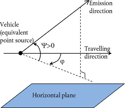
LW,0,dir is the directional sound power level of the specific noise (rolling, impact, squeal, braking, traction, aerodynamic, other effects) of a single vehicle in the directions ψ, φ defined with respect to the vehicle's direction of movement (see Figure [2.3.b]).
In the case of a stationary source, as during idling, it is assumed that the vehicle will remain for an overall time Tidle at a location within a track section with length L. Therefore, with Tref as the reference time period for the noise assessment (e.g. 12 hours, 4 hours, 8 hours), the directional sound power per unit length on that track section is defined by:

In general, directional sound power is obtained from each specific source as:
| LW,0,dir,i (ψ,φ) = LW,0,i + ΔLW,dir,vert,i + ΔLW,dir,hor,i | (2.3.5) |
where
ΔLW,dir,vert,i is the vertical directivity correction (dimensionless) function of ψ (Figure [2.3.b])
ΔLW,dir,hor,i is the horizontal directivity correction (dimensionless) function of φ (Figure [2.3.b]).
And where LW,0,dir,i(ψ,φ) shall, after being derived in 1/3 octave bands, be expressed in octave bands by energetically adding each pertaining 1/3 octave band together into the corresponding octave band.
For the purpose of the calculations, the source strength is then specifically expressed in terms of directional sound power per 1 m length of track LW′,tot,dir,i to account for the directivity of the sources in their vertical and horizontal direction, by means of the additional corrections.
Several LW,0,dir,i (ψ,φ) are considered for each vehicle-track-speed-running condition combination:
for a 1/3 octave frequency band ( i )
for each track section ( j )
source height ( h ) (for sources at 0,5 m h = 1, at 4,0 m h = 2)
directivity ( d ) of the source
A set of LW,0,dir,i (ψ,φ) are considered for each vehicle-track-speed-running condition combination, each track section, the heights corresponding to h = 1 and h = 2 and the directivity.
Rolling noise U.K.
The vehicle contribution and the track contribution to rolling noise are separated into four essential elements: wheel roughness, rail roughness, vehicle transfer function to the wheels and to the superstructure (vessels) and track transfer function. Wheel and rail roughness represent the cause of the excitation of the vibration at the contact point between the rail and the wheel, and the transfer functions are two empirical or modelled functions that represent the entire complex phenomena of the mechanical vibration and sound generation on the surfaces of the wheel, the rail, the sleeper and the track substructure. This separation reflects the physical evidence that roughness present on a rail may excite the vibration of the rail, but it will also excite the vibration of the wheel and vice versa. Not including one of these four parameters would prevent the decoupling of the classification of tracks and trains.
Wheel and rail roughness U.K.
Rolling noise is mainly excited by rail and wheel roughness in the wavelength range from 5-500 mm.
Definition U.K.
The roughness level Lr is defined as 10 times the logarithm to the base 10 of the square of the mean square value r2 of the roughness of the running surface of a rail or a wheel in the direction of motion (longitudinal level) measured in μm over a certain rail length or the entire wheel diameter, divided by the square of the reference value 

where
r 0
=
1 μm
r
=
r.m.s. of the vertical displacement difference of the contact surface to the mean level
The roughness level Lr is typically obtained as a spectrum of wavelength λ and it shall be converted to a frequency spectrum f = v/λ, where f is the centre band frequency of a given 1/3 octave band in Hz, λ is the wavelength in m, and v is the train speed in km/h. The roughness spectrum as a function of frequency shifts along the frequency axis for different speeds. In general cases, after conversion to the frequency spectrum by means of the speed, it is necessary to obtain new 1/3 octave band spectra values averaging between two corresponding 1/3 octave bands in the wavelength domain. To estimate the total effective roughness frequency spectrum corresponding to the appropriate train speed, the two corresponding 1/3 octave bands defined in the wavelength domain shall be averaged energetically and proportionally.
The rail roughness level (track side roughness) for the i-th wave-number band is defined as Lr,TR,i
By analogy, the wheel roughness level (vehicle side roughness) for the i-th wave-number band is defined as Lr,VEH,i .
The total and effective roughness level for wave-number band i (LR,tot,i ) is defined as the energy sum of the roughness levels of the rail and that of the wheel plus the A3(λ) contact filter to take into account the filtering effect of the contact patch between the rail and the wheel, and is in dB:

where expressed as a function of the i-th wave-number band corresponding to the wavelength λ.
The contact filter depends on the rail and wheel type and the load.
The total effective roughness for the j-th track section and each t-th vehicle type at its corresponding v speed shall be used in the method.
Vehicle, track and superstructure transfer function U.K.
Three speed-independent transfer functions, LH,TR,i LH,VEH,i and LH,VEH,SUP,i , are defined: the first for each j-th track section and the second two for each t-th vehicle type. They relate the total effective roughness level with the sound power of the track, the wheels and the superstructure respectively.
The superstructure contribution is considered only for freight wagons, therefore only for vehicle type ‘a’.
For rolling noise, therefore, the contributions from the track and from the vehicle are fully described by these transfer functions and by the total effective roughness level. When a train is idling, rolling noise shall be excluded.
For sound power per vehicle the rolling noise is calculated at axle height, and has as an input the total effective roughness level LR,TOT,i as a function of the vehicle speed v, the track, vehicle and superstructure transfer functions LH,TR,i , LH,VEH,i and LH,VEH,SUP,i , and the total number of axles Na :
for h = 1:
| LW,0,TR,i = LR,TOT,i + LH,TR,i + 10 × lg(Na ) | dB | (2.3.8) |
| LW,0,VEH,i = LR,TOT,i + LH,VEH,i + 10 × lg(Na ) | dB | (2.3.9) |
| LW,0,VEHSUP,i = LR,TOT,i + LH,VEHSUP,i + 10 × lg(Na ) | dB | (2.3.10) |
where Na is the number of axles per vehicle for the t-th vehicle type.

A minimum speed of 50 km/h (30 km/h only for trams and light metro) shall be used to determine the total effective roughness and therefore the sound power of the vehicles (this speed does not affect the vehicle flow calculation) to compensate for the potential error introduced by the simplification of rolling noise definition, braking noise definition and impact noise from crossings and switches definition.
Impact noise (crossings, switches and junctions) U.K.
Impact noise can be caused by crossings, switches and rail joints or points. It can vary in magnitude and can dominate rolling noise. Impact noise shall be considered for jointed tracks. For impact noise due to switches, crossings and joints in track sections with a speed of less than 50 km/h (30 km/h only for trams and light metro), since the minimum speed of 50 km/h (30 km/h only for trams and light metro) is used to include more effects according to the description of the rolling noise chapter, modelling shall be avoided. Impact noise modelling shall also be avoided under running condition c = 2 (idling).
Impact noise is included in the rolling noise term by (energy) adding a supplementary fictitious impact roughness level to the total effective roughness level on each specific j-th track section where it is present. In this case a new LR,TOT + IMPACT,i shall be used in place of LR,TOT,i and it will then become:

LR,IMPACT,i is a 1/3 octave band spectrum (as a function of frequency). To obtain this frequency spectrum, a spectrum is given as a function of wavelength λ and shall be converted to the required spectrum as a function of frequency using the relation λ = v/f, where f is the 1/3 octave band centre frequency in Hz and v is the s-th vehicle speed of the t-th vehicle type in km/h.
Impact noise will depend on the severity and number of impacts per unit length or joint density, so in the case where multiple impacts are given, the impact roughness level to be used in the equation above shall be calculated as follows:

where LR,IMPACT–SINGLE,i is the impact roughness level as given for a single impact and nl is the joint density.
The default impact roughness level is given for a joint density nl = 0,01 m–1, which is one joint per each 100 m of track. Situations with different numbers of joints shall be approximated by adjusting the joint density nl . It should be noted that when modelling the track layout and segmentation, the rail joint density shall be taken into account, i.e. it may be necessary to take a separate source segment for a stretch of track with more joints. The LW,0 of track, wheel/bogie and superstructure contribution are incremented by means of the LR,IMPACT,i for +/– 50 m before and after the rail joint. In the case of a series of joints, the increase is extended to between – 50 m before the first joint and + 50 m after the last joint.
The applicability of these sound power spectra shall normally be verified on-site.
For jointed tracks, a default nl of 0,01 shall be used.
Squeal U.K.
Curve squeal is a special source that is only relevant for curves and is therefore localised. As it can be significant, an appropriate description is required. Curve squeal is generally dependent on curvature, friction conditions, train speed and track-wheel geometry and dynamics. The emission level to be used is determined for curves with radius below or equal to 500 m and for sharper curves and branch-outs of points with radii below 300 m. The noise emission should be specific to each type of rolling stock, as certain wheel and bogie types may be significantly less prone to squeal than others.
The applicability of these sound power spectra shall normally be verified on-site, especially for trams.
Taking a simple approach, squeal noise shall be considered by adding 8 dB for R < 300 m and 5 dB for 300 m < R < 500 m to the rolling noise sound power spectra for all frequencies. Squeal contribution shall be applied on railway track sections where the radius is within the ranges mentioned above for at least a 50 m length of track.
Traction noise U.K.
Although traction noise is generally specific to each characteristic operating condition amongst constant speed, deceleration, acceleration and idling, the only two conditions modelled are constant speed (that is valid as well when the train is decelerating or when it is accelerating) and idling. The source strength modelled only corresponds to maximum load conditions and this results in the quantities LW,0,const,i = LW,0,idling,i . Also, the LW,0,idling,i corresponds to the contribution of all physical sources of a given vehicle attributable to a specific height, as described in 2.3.1.
The LW,0,idling,i is expressed as a static noise source in the idling position, for the duration of the idling condition, and to be used modelled as a fixed point source as described in the following chapter for industrial noise. It shall be considered only if trains are idling for more than 0,5 hours.
These quantities can either be obtained from measurements of all sources at each operating condition, or the partial sources can be characterised individually, determining their parameter dependency and relative strength. This may be done by means of measurements on a stationary vehicle, by varying shaft speeds of the traction equipment, following ISO 3095:2005. As far as relevant, several traction noise sources have to be characterised which might not be all directly depending on the train speed:
noise from the power train, such as diesel engines (including inlet, exhaust and engine block), gear transmission, electrical generators, mainly dependent on engine round per minute speed (rpm), and electrical sources such as converters, which may be mostly load-dependent,
noise from fans and cooling systems, depending on fan rpm; in some cases fans can be directly coupled to the driveline,
intermittent sources such as compressors, valves and others with a characteristic duration of operation and corresponding duty cycle correction for the noise emission.
As each of these sources can behave differently at each operating condition, the traction noise shall be specified accordingly. The source strength is obtained from measurements under controlled conditions. In general, locomotives will tend to show more variation in loading as the number of vehicles hauled and thereby the power output can vary significantly, whereas fixed train formations such as electric motored units (EMUs), diesel motored units (DMUs) and high-speed trains have a better defined load.
There is no a priori attribution of the source sound power to the source heights, and this choice shall depend on the specific noise and vehicle assessed. It shall be modelled to be at source A (h = 1) and at source B (h = 2).
Aerodynamic noise U.K.
Aerodynamic noise is only relevant at high speeds above 200 km/h and therefore it should first be verified whether it is actually necessary for application purposes. If the rolling noise roughness and transfer functions are known, it can be extrapolated to higher speeds and a comparison can be made with existing high-speed data to check whether higher levels are produced by aerodynamic noise. If train speeds on a network are above 200 km/h but limited to 250 km/h, in some cases it may not be necessary to include aerodynamic noise, depending on the vehicle design.
The aerodynamic noise contribution is given as a function of speed:
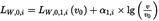

where
v 0 is a speed at which aerodynamic noise is dominant and is fixed at 300 km/h
LW,0,1,i is a reference sound power determined from two or more measurement points, for sources at known source heights, for example the first bogie
LW,0,2,i is a reference sound power determined from two or more measurement points, for sources at known source heights, for example the pantograph recess heights
α1,i is a coefficient determined from two or more measurement points, for sources at known source heights, for example the first bogie
α2,i is a coefficient determined from two or more measurement points, for sources at known source heights, for example the pantograph recess heights.
Source directivity U.K.
The horizontal directivity ΔLW,dir,hor,i in dB is given in the horizontal plane and by default can be assumed to be a dipole for rolling, impact (rail joints etc.), squeal, braking, fans and aerodynamic effects, given for each i-th frequency band by:
| ΔLW,dir,hor,i = 10 × lg(0,01 + 0,99 · sin2 φ) | (2.3.15) |
The vertical directivity ΔLW,dir,ver,i in dB is given in the vertical plane for source A (h = 1), as a function of the centre band frequency fc,i of each i-th frequency band, and for – π/2 < ψ < π/2 by:

For source B (h = 2) for the aerodynamic effect:
| ΔLW,dir,ver,i = 10 × lg(cos2 ψ) | for ψ < 0 | (2.3.17) |
ΔLW,dir,ver,i = 0 elsewhere
Directivity ΔLdir,ver,i is not considered for source B (h = 2) for other effects, as omni-directionality is assumed for these sources in this position.
2.3.3. Additional effects U.K.
Correction for structural radiation (bridges and viaducts) U.K.
In the case where the track section is on a bridge, it is necessary to consider the additional noise generated by the vibration of the bridge as a result of the excitation caused by the presence of the train. Because it is not simple to model the bridge emission as an additional source, given the complex shapes of bridges, an increase in the rolling noise is used to account for the bridge noise. The increase shall be modelled exclusively by adding a fixed increase in the noise sound power per each third octave band. The sound power of only the rolling noise is modified when considering the correction and the new LW,0,rolling–and–bridge,i shall be used instead of LW,0,rolling-only,i :
| LW,0,rolling–and–bridge,i = LW,0,rolling–only,i + Cbridge | dB | (2.3.18) |
where Cbridge is a constant that depends on the bridge type, and LW,0,rolling–only,i is the rolling noise sound power on the given bridge that depends only on the vehicle and track properties.
Correction for other railway-related noise sources U.K.
Various sources like depots, loading/unloading areas, stations, bells, station loudspeakers, etc. can be present and are associated with the railway noise. These sources are to be treated as industrial noise sources (fixed noise sources) and shall be modelled, if relevant, according to the following chapter for industrial noise.
2.4. Industrial noise U.K.
2.4.1. Source description U.K.
Classification of source types (point, line, area) U.K.
The industrial sources are of very variable dimensions. They can be large industrial plants as well as small concentrated sources like small tools or operating machines used in factories. Therefore, it is necessary to use an appropriate modelling technique for the specific source under assessment. Depending on the dimensions and the way several single sources extend over an area, with each belonging to the same industrial site, these may be modelled as point sources, source lines or area sources. In practice, the calculations of the noise effect are always based on point sources, but several point sources can be used to represent a real complex source, which mainly extends over a line or an area.
Number and position of equivalent sound sources U.K.
The real sound sources are modelled by means of equivalent sound sources represented by one or more point sources so that the total sound power of the real source corresponds to the sum of the single sound powers attributed to the different point sources.
The general rules to be applied in defining the number of point sources to be used are:
line or surface sources where the largest dimension is less than 1/2 of the distance between the source and the receiver can be modelled as single point sources,
sources where the largest dimension is more than 1/2 of the distance between the source and the receiver should be modelled as a series of incoherent point sources in a line or as a series of incoherent point sources over an area, such that for each of these sources the condition of 1/2 is fulfilled. The distribution over an area can include vertical distribution of point sources,
for sources where the largest dimensions in height are over 2 m or near the ground, special care should be administered to the height of the source. Doubling the number of sources, redistributing them only in the z-component, may not lead to a significantly better result for this source,
in the case of any source, doubling the number of sources over the source area (in all dimensions) may not lead to a significantly better result.
The position of the equivalent sound sources cannot be fixed, given the large number of configurations that an industrial site can have. Best practices will normally apply.
Sound power emission U.K.
General U.K.
The following information constitutes the complete set of input data for sound propagation calculations with the methods to be used for noise mapping:
Emitted sound power level spectrum in octave bands
Working hours (day, evening, night, on a yearly averaged basis)
Location (coordinates x, y) and elevation (z) of the noise source
Type of source (point, line, area)
Dimensions and orientation
Operating conditions of the source
Directivity of the source.
The point, line and area source sound power are required to be defined as:
For a point source, sound power LW and directivity as a function of the three orthogonal coordinates (x, y, z);
Two types of source lines can be defined:
source lines representing conveyor belts, pipe lines, etc., sound power per metre length LW′ and directivity as a function of the two orthogonal coordinates to the axis of the source line,
source lines representing moving vehicles, each associated with sound power LW and directivity as a function of the two orthogonal coordinates to the axis of the source line and sound power per metre LW′ derived by means of the speed and number of vehicles travelling along this line during day, evening and night; The correction for the working hours, to be added to the source sound power to define the corrected sound power that is to be used for calculations over each time period, CW in dB is calculated as follows:
Where:
VSpeed of the vehicle [km/h];
nNumber of vehicles passages per period [-];
lTotal length of the source [m].
For an area source, sound power per square metre LW/m2 , and no directivity (may be horizontal or vertical).

The working hours are an essential input for the calculation of noise levels. The working hours shall be given for the day, evening and night period and, if the propagation is using different meteorological classes defined during each of the day, night and evening periods, then a finer distribution of the working hours shall be given in sub-periods matching the distribution of meteorological classes. This information shall be based on a yearly average.
The correction for the working hours, to be added to the source sound power to define the corrected sound power that shall be used for calculations over each time period, CW in dB is calculated as follows:

where
T is the active source time per period based on a yearly averaged situation, in hours;
Tref is the reference period of time in hours (e.g. day is 12 hours, evening is 4 hours, night is 8 hours).
For the more dominant sources, the yearly average working hours correction shall be estimated at least within 0,5 dB tolerance in order to achieve an acceptable accuracy (this is equivalent to an uncertainty of less than 10 % in the definition of the active period of the source).
Source directivity U.K.
The source directivity is strongly related to the position of the equivalent sound source next to nearby surfaces. Because the propagation method considers the reflection of the nearby surface as well its sound absorption, it is necessary to consider carefully the location of the nearby surfaces. In general, these two cases will always be distinguished:
a source sound power and directivity is determined and given relative to a certain real source when this is in free field (excluding the terrain effect). This is in agreement with the definitions concerning the propagation, if it is assumed that there is no nearby surface less than 0,01 m from the source and surfaces at 0,01 m or more are included in the calculation of the propagation,
a source sound power and directivity is determined and given relative to a certain real source when this is placed in a specific location and therefore the source sound power and directivity is in fact an ‘equivalent’ one, since it includes the modelling of the effect of the nearby surfaces. This is defined in ‘semi-free field’ according to the definitions concerning the propagation. In this case, the nearby surfaces modelled shall be excluded from the calculation of propagation.
The directivity shall be expressed in the calculation as a factor ΔLW,dir,xyz (x, y, z) to be added to the sound power to obtain the right directional sound power of a reference sound source seen by the sound propagation in the direction given. The factor can be given as a function of the direction vector defined by (x,y,z) with 
2.5. Calculation of noise propagation for road, railway, industrial sources. U.K.
2.5.1. Scope and applicability of the method U.K.
This document specifies a method for calculating the attenuation of noise during its outdoor propagation. Knowing the characteristics of the source, this method predicts the equivalent continuous sound pressure level at a receiver point corresponding to two particular types of atmospheric conditions:
downward-refraction propagation conditions (positive vertical gradient of effective sound celerity) from the source to the receiver,
homogeneous atmospheric conditions (null vertical gradient of effective sound celerity) over the entire area of propagation.
The method of calculation described in this document applies to industrial infrastructures and land transport infrastructures. It therefore applies in particular to road and railway infrastructures. Aircraft transport is included in the scope of the method only for the noise produced during ground operations and excludes take-off and landing.
Industrial infrastructures that emit impulsive or strong tonal noises as described in ISO 1996-2:2007 do not fall within the scope of this method.
The method of calculation does not provide results in upward-refraction propagation conditions (negative vertical gradient of effective sound speed) but these conditions are approximated by homogeneous conditions when computing Lden.
To calculate the attenuation due to atmospheric absorption in the case of transport infrastructure, the temperature and humidity conditions are calculated according to ISO 9613-1:1996.
The method provides results per octave band, from 63 Hz to 8 000 Hz. The calculations are made for each of the centre frequencies.
Partial covers and obstacles sloping, when modelled, more than 15° in relation to the vertical are out of the scope of this calculation method.
A single screen is calculated as a single diffraction calculation, two or more screens in a single path are treated as a subsequent set of single diffractions by applying the procedure described further.
2.5.2. Definitions used U.K.
All distances, heights, dimensions and altitudes used in this document are expressed in metres (m).
The notation MN stands for the distance in 3 dimensions (3D) between the points M and N, measured according to a straight line joining these points.
The notation M̂N stands for the curved path length between the points M and N, in favourable conditions.
It is customary for real heights to be measured vertically in a direction perpendicular to the horizontal plane. Heights of points above the local ground are denoted h, absolute heights of points and absolute height of the ground are to be noted by the letter H.
To take into account the actual relief of the land along a propagation path, the notion of ‘equivalent height’ is introduced, to be noted by the letter z. This substitutes real heights in the ground effect equations.
The sound levels, noted by the capital letter L, are expressed in decibels (dB) per frequency band when index A is omitted. The sound levels in decibels dB(A) are given the index A.
The sum of the sound levels due to mutually incoherent sources is noted by the sign ⊕ in accordance with the following definition:
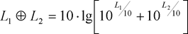 | (2.5.1) |
2.5.3. Geometrical considerations U.K.
Source segmentation U.K.
Real sources are described by a set of point sources or, in the case of railway traffic or road traffic, by incoherent source lines. The propagation method assumes that line or area sources have previously been split up to be represented by a series of equivalent point sources. This may have occurred as pre-processing of the source data, or may occur within the pathfinder component of the calculation software. The means by which this has occurred is outside the scope of the current methodology.
Propagation paths U.K.
The method operates on a geometrical model consisting of a set of connected ground and obstacles surfaces. A vertical propagation path is deployed on one or more vertical planes with respect to the horizontal plane. For trajectories including reflections onto vertical surfaces not orthogonal to the incident plane, another vertical plane is subsequently considered including the reflected part of the propagation path. In these cases, where more vertical planes are used to describe the entire trajectory from the source to the receiver, the vertical planes are then flattened, like an unfolding Chinese screen.
Significant heights above the ground U.K.
The equivalent heights are obtained from the mean ground plane between the source and the receiver. This replaces the actual ground with a fictitious plane representing the mean profile of the land.

1
:
Actual relief
2
:
Mean plane
The equivalent height of a point is its orthogonal height in relation to the mean ground plane. The equivalent source height zs and the equivalent receiver height zr can therefore be defined. The distance between the source and receiver in projection over the mean ground plane is noted by dp .
If the equivalent height of a point becomes negative, i.e. if the point is located below the mean ground plane, a null height is retained, and the equivalent point is then identical with its possible image.
Calculation of the mean plane U.K.
In the plane of the path, the topography (including terrain, mounds, embankments and other man-made obstacles, buildings, …) may be described by an ordered set of discrete points (xk, Hk ); k є {1,…,n}. This set of points defines a polyline, or equivalently, a sequence of straight segments Hk = akx + bk, x є [xk, xk + 1 ]; k є {1,…n}, where:
| ak = (Hk + 1 – Hk )/(xk + 1 – xk ) | (2.5.2) | |
| bk = (Hk · xk + 1 – Hk + 1 · xk )/(xk + 1 – xk ) |
The mean plane is represented by the straight line Z = ax + b; x є [x 1, xn ], which is adjusted to the polyline by means of a least-square approximation. The equation of the mean line can be worked out analytically.
Using:


The coefficients of the straight line are given by:


Where segments with xk + 1 = xk shall be ignored when evaluating eq. 2.5.3.
Reflections by building façades and other vertical obstacles U.K.
Contributions from reflections are taken into account by the introduction of image sources as described further.
2.5.4. Sound propagation model U.K.
For a receiver R the calculations are made according to the following steps:
(1)
on each propagation path:
calculation of the attenuation in favourable conditions,
calculation of the attenuation in homogeneous conditions,
calculation of the long-term sound level for each path;
(2)
accumulation of the long-term sound levels for all paths affecting a specific receiver, therefore allowing the total sound level to be calculated at the receiver point.
It should be noted that only the attenuations due to the ground effect (Aground ) and diffraction (Adif ) are affected by meteorological conditions.
2.5.5. Calculation process U.K.
For a point source S of directional sound power Lw,0,dir and for a given frequency band, the equivalent continuous sound pressure level at a receiver point R in given atmospheric conditions is obtained according to the equations following below.
Sound level in favourable conditions (LF) for a path (S,R) U.K.
| LF = LW,0,dir – AF | (2.5.5) |
The term AF represents the total attenuation along the propagation path in favourable conditions, and is broken down as follows:
| LF = Adiv + Aatm + Aboundary,F | (2.5.6) |
where
Adiv is the attenuation due to geometrical divergence;
Aatm is the attenuation due to atmospheric absorption;
Aboundary,F is the attenuation due to the boundary of the propagation medium in favourable conditions. It may contain the following terms:
Aground,F which is the attenuation due to the ground in favourable conditions;
Adif,F which is the attenuation due to diffraction in favourable conditions.
For a given path and frequency band, the following two scenarios are possible:
either Aground,F is calculated with no diffraction (Adif,F = 0 dB) and Aboundary,F = Aground,F ;
or Adif,F is calculated. The ground effect is taken into account in the Adif,F equation itself (Aground,F = 0 dB). This therefore gives Aboundary,F = Adif,F .
Sound level in homogeneous conditions (LH) for a path (S,R) U.K.
The procedure is strictly identical to the case of favourable conditions presented in the previous section.
| LH = LW,0,dir – AH | (2.5.7) |
The term AH represents the total attenuation along the propagation path in homogeneous conditions and is broken down as follows:
| AH = Adiv + Aatm + Aboundary,H | (2.5.8) |
where
Adiv is the attenuation due to geometrical divergence;
Αatm is the attenuation due to atmospheric absorption;
Aboundary,H is the attenuation due to the boundary of the propagation medium in homogeneous conditions. It may contain the following terms:
Αground,H which is the attenuation due to the ground in homogeneous conditions;
Adif,H which is the attenuation due to diffraction in homogeneous conditions.
For a given path and frequency band, the following two scenarios are possible:
either Αground,H (Adif,H = 0 dB) is calculated with no diffraction and Aboundary,H = Αground,H ;
or Adif,H (Αground,H = 0 dB) is calculated. The ground effect is taken into account in the Adif,H equation itself. This therefore gives Aboundary,H = Adif,H
Statistical approach inside urban areas for a path (S,R) U.K.
Inside urban areas, a statistical approach to the calculation of the sound propagation behind the first line of buildings is also allowed, provided that such a method is duly documented, including relevant information on the quality of the method. This method may replace the calculation of the Aboundary,H and Aboundary,F by an approximation of the total attenuation for the direct path and all reflections. The calculation will be based on the average building density and the average height of all buildings in the area.
Long-term sound level for a path (S,R) U.K.
The ‘long-term’ sound level along a path starting from a given point source is obtained from the logarithmic sum of the weighted sound energy in homogeneous conditions and the sound energy in favourable conditions.
These sound levels are weighted by the mean occurrence p of favourable conditions in the direction of the path (S,R):

NB: The occurrence values for p are expressed in percentages. So for example, if the occurrence value is 82 %, equation (2.5.9) would have p = 0,82.U.K.
Long-term sound level at point R for all paths U.K.
The total long-term sound level at the receiver for a frequency band is obtained by energy summing contributions from all N paths, all types included:

where
n is the index of the paths between S and R.
Taking reflections into account by means of image sources is described further. The percentage of occurrences of favourable conditions in the case of a path reflected on a vertical obstacle is taken to be identical to the occurrence of the direct path.
If S′ is the image source of S, then the occurrence p′ of the path (S′,R) is taken to be equal to the occurrence p of the path (Si,R).
Long-term sound level at point R in decibels A (dBA) U.K.
The total sound level in decibels A (dBA) is obtained by summing levels in each frequency band:

where i is the index of the frequency band. AWC is the A-weighting correction according to the international standard IEC 61672-1:2003.
This level LAeq,LT constitutes the final result, i.e. the long-term A-weighted sound pressure level at the receiver point on a specific reference time interval (e.g. day or evening, or night or a shorter time during day, evening or night).
2.5.6. Calculation of noise propagation for road, railway, industrial sources. U.K.
Geometrical divergence U.K.
The attenuation due to geometrical divergence, Adiv, corresponds to a reduction in the sound level due to the propagation distance. For a point sound source in free field, the attenuation in dB is given by:
| Adiv = 20 × lg(d) + 11 | (2.5.12) |
where d is the direct 3D slant distance between the source and the receiver.
Atmospheric absorption U.K.
The attenuation due to atmospheric absorption Aatm during propagation over a distance d is given in dB by the equation:
| Aatm = αatm · d/1 000 | (2.5.13) |
where
d is the direct 3D slant distance between the source and the receiver in m;
αatm is the atmospheric attenuation coefficient in dB/km at the nominal centre frequency for each frequency band, in accordance with ISO 9613-1.
The values of the αatm coefficient are given for a temperature of 15 °C, a relative humidity of 70 % and an atmospheric pressure of 101 325 Pa. They are calculated with the exact centre frequencies of the frequency band. These values comply with ISO 9613-1. Meteorological average over the long term shall be used if meteorological data is available.
Ground effect U.K.
The attenuation due to the ground effect is mainly the result of the interference between the reflected sound and the sound that is propagated directly from the source to the receiver. It is physically linked to the acoustic absorption of the ground above which the sound wave is propagated. However, it is also significantly dependent on atmospheric conditions during propagation, as ray bending modifies the height of the path above the ground and makes the ground effects and land located near the source more or less significant.
In case the propagation between the source and the receiver is affected by any obstacle in the propagation plane, the ground effect is calculated separately on the source and receiver side. In this case, zs and zr refer to the equivalent source and/or receiver position as indicated further where the calculation of the diffraction Adif is presented.
Acoustic characterisation of ground U.K.
The acoustic absorption properties of the ground are mainly linked to its porosity. Compact ground is generally reflective and porous ground is absorbent.
For operational calculation requirements, the acoustic absorption of a ground is represented by a dimensionless coefficient G, between 0 and 1. G is independent of the frequency. Table 2.5.a gives the G values for the ground outdoors. In general, the average of the coefficient G over a path takes values between 0 and 1.
Table 2.5.a
G values for different types of ground
| Description | Type | (kPa · s/m2) | G value |
|---|---|---|---|
| Very soft (snow or moss-like) | A | 12,5 | 1 |
| Soft forest floor (short, dense heather-like or thick moss) | B | 31,5 | 1 |
| Uncompacted, loose ground (turf, grass, loose soil) | C | 80 | 1 |
| Normal uncompacted ground (forest floors, pasture field) | D | 200 | 1 |
| Compacted field and gravel (compacted lawns, park area) | E | 500 | 0,7 |
| Compacted dense ground (gravel road, car park) | F | 2 000 | 0,3 |
| Hard surfaces (most normal asphalt, concrete) | G | 20 000 | 0 |
| Very hard and dense surfaces (dense asphalt, concrete, water) | H | 200 000 | 0 |
Gpath is defined as the fraction of absorbent ground present over the entire path covered.
When the source and receiver are close-by so that dp ≤ 30(zs + zr ), the distinction between the type of ground located near the source and the type of ground located near the receiver is negligible. To take this comment into account, the ground factor Gpath is therefore ultimately corrected as follows:

where Gs is the ground factor of the source area. Gs = 0 for road platforms(1), slab tracks. Gs = 1 for rail tracks on ballast. There is no general answer in the case of industrial sources and plants.
G may be linked to the flow resistivity.


The following two subsections on calculations in homogeneous and favourable conditions introduce the generic Ḡw and Ḡm notations for the absorption of the ground. Table 2.5.b gives the correspondence between these notations and the Gpath and G′path variables.
Table 2.5.b
Correspondence between Ḡw and Ḡm and (Gpath , G′path )
| Homogeneous conditions | Favourable conditions | |||||
|---|---|---|---|---|---|---|
| Aground | Δground(S,O) | Δground(O,R) | Ag round | Δground(S,O) | Δground(O,R) | |
| Ḡw | G′path | Gpath | ||||
| Ḡm | G′path | Gpath | G′path | Gpath | ||
Calculations in homogeneous conditions U.K.
The attenuation due to the ground effect in homogeneous conditions is calculated according to the following equations:
if Gpath ≠ 0

where

fm is the nominal centre frequency of the frequency band considered, in Hz, c is the speed of the sound in the air, taken as equal to 340 m/s, and Cf is defined by:

where the values of w are given by the equation below:
 | (2.5.17) |
Ḡw may be equal to either Gpath or G′path depending on whether the ground effect is calculated with or without diffraction, and according to the nature of the ground under the source (real source or diffracted). This is specified in the following subsections and summarised in Table 2.5.b.
 | (2.5.18) |
is the lower bound of Aground,H .
For a path (Si,R) in homogeneous conditions without diffraction:
Ḡw = G′path
Ḡm = G′path
With diffraction, refer to the section on diffraction for the definitions of Ḡw and Ḡm .
if Gpath = 0: Aground,H = – 3 dB
The term – 3(1 – Ḡm ) takes into account the fact that when the source and the receiver are far apart, the first reflection source side is no longer on the platform but on natural land.
Calculation in favourable conditions U.K.
The ground effect in favourable conditions is calculated with the equation of Aground,H , provided that the following modifications are made:
If Gpath ≠ 0
If Gpath = 0
Aground,F = Aground,F,min


The height corrections δ zs and δ zr convey the effect of the sound ray bending. δ zT accounts for the effect of the turbulence.
Ḡm may also be equal to either Gpath or G′path depending on whether the ground effect is calculated with or without diffraction, and according to the nature of the ground under the source (real source or diffracted). This is specified in the following subsections.
For a path (Si,R) in favourable conditions without diffraction:
Ḡw = Gpath in equation (2.5.17);
Ḡm = G′path .
With diffraction, refer to the next section for the definitions of Ḡw and Ḡm .
Diffraction U.K.
As a general rule, the diffraction shall be studied at the top of each obstacle located on the propagation path. If the path passes ‘high enough’ over the diffraction edge, Adif = 0 can be set and a direct view calculated, in particular by evaluating Aground .
In practice, for each frequency band centre frequency, the path difference δ is compared with the quantity – λ/20. If an obstacle does not produce diffraction, this for instance being determined according to Rayleigh's criterion, there is no need to calculate Adif for the frequency band considered. In other words, Adif = 0 in this case. Otherwise, Adif is calculated as described in the remainder of this part. This rule applies in both homogeneous and favourable conditions, for both single and multiple diffraction.
When, for a given frequency band, a calculation is made according to the procedure described in this section, Aground is set as equal to 0 dB when calculating the total attenuation. The ground effect is taken into account directly in the general diffraction calculation equation.
The equations proposed here are used to process the diffraction on thin screens, thick screens, buildings, earth berms (natural or artificial), and by the edges of embankments, cuttings and viaducts.
When several diffracting obstacles are encountered on a propagation path, they are treated as a multiple diffraction by applying the procedure described in the following section on calculation of the path difference.
The procedures presented here are used to calculate the attenuations in both homogeneous conditions and favourable conditions. Ray bending is taken into account in the calculation of the path difference and to calculate the ground effects before and after diffraction.
General principles U.K.
Figure 2.5.c illustrates the general method of calculation of the attenuation due to diffraction. This method is based on breaking down the propagation path into two parts: the ‘source side’ path, located between the source and the diffraction point, and the ‘receiver side’ path, located between the diffraction point and the receiver.
The following are calculated:
a ground effect, source side, Δ ground(S,O)
a ground effect, receiver side, Δ ground(O,R)
and three diffractions:
between the source S and the receiver R: Δ dif(S,R)
between the image source S′ and R: Δ dif(S′,R)
between S and the image receiver R′: Δ dif(S,R′) .
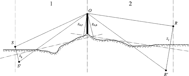
1
:
Source side
2
:
Receiver side
where
S is the source;
R is the receiver;
S′ is the image source in relation to the mean ground plane source side;
R′ is the image receiver in relation to the mean ground plane receiver side;
O is the diffraction point;
z s is the equivalent height of the source S in relation to the mean plane source side;
z o,s is the equivalent height of the diffraction point O in relation to the mean ground plane source side;
z r is the equivalent height of the receiver R in relation to the mean plane receiver side;
z o,r is the equivalent height of the diffraction point O in relation to the mean ground plane receiver side.
The irregularity of the ground between the source and the diffraction point, and between the diffraction point and the receiver, is taken into account by means of equivalent heights calculated in relation to the mean ground plane, source side first and receiver side second (two mean ground planes), according to the method described in the subsection on significant heights above the ground.
Pure diffraction U.K.
For pure diffraction, with no ground effects, the attenuation is given by:

where
| Ch = 1 | (2.5.22) |
λ is the wavelength at the nominal centre frequency of the frequency band considered;
δ is the path difference between the diffracted path and the direct path (see next subsection on calculation of the path difference);
C″ is a coefficient used to take into account multiple diffractions:
C″ = 1 for a single diffraction.
For a multiple diffraction, if e is the total distance along the path, O1 to O2 + O2 to O3 + O3 to O4 from the ‘rubber band method’, (see Figures 2.5.d and 2.5.f) and if e exceeds 0,3 m (otherwise C″ = 1), this coefficient is defined by:
 | (2.5.23) |
The values of Δdif shall be bound:
if Δ dif < 0: Δ dif = 0 dB
if Δ dif > 25: Δ dif = 25 dB for a diffraction on a horizontal edge and only on the term Δdif which figures in the calculation of Adif . This upper bound shall not be applied in the Δdif terms that intervene in the calculation of Δ ground , or for a diffraction on a vertical edge (lateral diffraction) in the case of industrial noise mapping.
Calculation of the path difference U.K.
The path difference δ is calculated in a vertical plane containing the source and the receiver. This is an approximation in relation to the Fermat principle. The approximation remains applicable here (source lines). The path difference δ is calculated as in the following Figures, based on the situations encountered.
Homogeneous conditions U.K.
Figure 2.5.d
Calculation of the path difference in homogeneous conditions. O, O1 , and O2 are the diffraction points
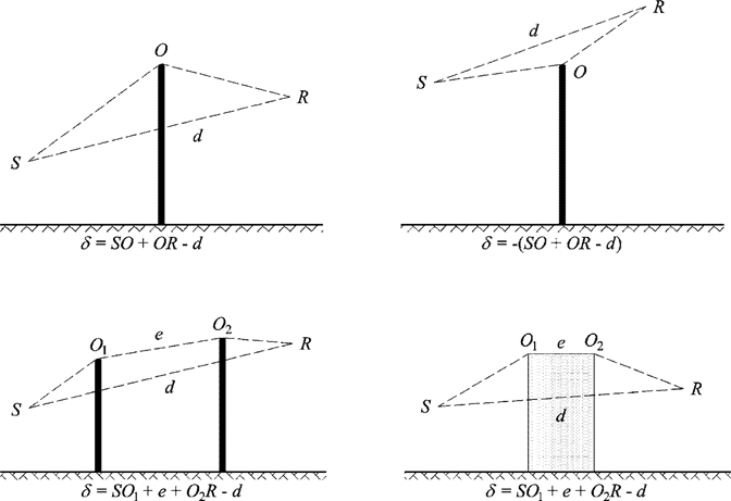
Note: For each configuration, the expression of δ is given.U.K.
Favourable conditions U.K.
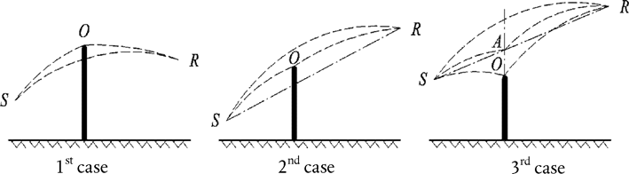
In favourable conditions, it is considered that the three curved sound rays SO, OR, and SR have an identical radius of curvature Γ defined by:
| Γ = max(1 000,8d) | (2.5.24) |
The length of a sound ray curve MN is noted M̂N in favourable conditions. This length is equal to:
 | (2.5.25) |
In principle, three scenarios should be considered in the calculation of the path difference in favourable conditions δF (see Figure 2.5.e). In practice, two equations are sufficient:
if the straight sound ray SR is masked by the obstacle (1st and 2nd case in Figure 2.5.e):
(2.5.26) if the straight sound ray SR is not masked by the obstacle (3rd case in Figure 2.5.e):
(2.5.27)


where A is the intersection of the straight sound ray SR and the extension of the diffracting obstacle.
For the multiple diffractions in favourable conditions:
determine the convex hull defined by the various potential diffraction edges;
eliminate the diffraction edges which are not on the boundary of the convex hull;
calculate δF based on the lengths of the curved sound ray, by breaking down the diffracted path into as many curved segments as necessary (see Figure 2.5.f)
(2.5.28)

Figure 2.5.f
Example of calculation of the path difference in favourable conditions, in the case of multiple diffractions

In the scenario presented in Figure 2.5.f, the path difference is:
 | (2.5.29) |
Calculation of the attenuation Adif U.K.
The attenuation due to diffraction, taking the ground effects on the source side and receiver side into account, is calculated according to the following general equations:

where
Δ dif (S,R) is the attenuation due to the diffraction between the source S and the receiver R
Δ ground(S,O) is the attenuation due to the ground effect on the source side, weighted by the diffraction on the source side; where it is understood that O = O1 in case of multiple diffractions as in Figure 2.5.f
Δ ground(O,R) is the attenuation due to the ground effect on the receiver side, weighted by the diffraction on the receiver side (see the following subsection on calculation of the term Δ ground(O,R) ).
Calculation of the term Δ ground(S,O) U.K.
 | (2.5.31) |
where
Aground(S,O) is the attenuation due to the ground effect between the source S and the diffraction point O. This term is calculated as indicated in the previous subsection on calculations in homogeneous conditions and in the previous subsection on calculation in favourable conditions, with the following hypotheses:
zr = zo,s ,
Gpath is calculated between S and O,
In homogeneous conditions: Ḡw = G′path in equation (2.5.17), Ḡm = G′path in equation (2.5.18),
In favourable conditions: Ḡw = Gpath in equation (2.5.17), Ḡm = G′path in equation (2.5.20),
Δ dif(S′,R) is the attenuation due to the diffraction between the image source S′ and R, calculated as in the previous subsection on pure diffraction,
Δ dif(S,R) is the attenuation due to the diffraction between S and R, calculated as in Subsection VI.4.4.b.
Calculation of the term Δ ground(O,R) U.K.
 | (2.5.32) |
where
Aground (O,R) is the attenuation due to the ground effect between the diffraction point O and the receiver R. This term is calculated as indicated in the previous subsection on calculation in homogeneous conditions and in the previous subsection on calculation in favourable conditions, with the following hypotheses:
zs = zo,r
Gpath is calculated between O and R.
The G′path correction does not need to be taken into account here as the source considered is the diffraction point. Therefore, Gpath shall indeed be used in the calculation of ground effects, including for the lower bound term of the equation which becomes – 3(1 – Gpath ).
In homogeneous conditions, Ḡw = Gpath in equation (2.5.17) and Ḡm = Gpath in equation (2.5.18);
In favourable conditions, Ḡw = Gpath in equation (2.5.17) and Ḡm = Gpath in equation (2.5.20);
Δ dif(S,R′) is the attenuation due to the diffraction between S and the image receiver R′, calculated as in the previous section on pure diffraction;
Δ dif(S,R) is the attenuation due to the diffraction between S and R, calculated as in the previous subsection on pure diffraction.
Vertical edge scenarios U.K.
Equation (2.5.21) may be used to calculate the diffractions on vertical edges (lateral diffractions) in case of industrial noise. If this is the case, Adif = Δ dif(S,R) is taken and the term Aground is kept. In addition, Aatm and Aground shall be calculated from the total length of the propagation path. Adiv is still calculated from the direct distance d. Equations (2.5.8) and (2.5.6) respectively become:


Δ dif is indeed used in homogeneous conditions in equation (2.5.34).
Reflections on vertical obstacles U.K.
Attenuation through absorption U.K.
The reflections on vertical obstacles are dealt with by means of image sources. Reflections on building façades and noise barriers are thus treated in this way.
An obstacle is considered to be vertical if its slope in relation to the vertical is less than 15°.
When dealing with reflections on objects which slope in relation to the vertical is more or equal to 15° the object is not considered.
The obstacles where at least one dimension is less than 0,5 m shall be ignored in the reflection calculation, except for special configurations(2).
Note that reflections on the ground are not dealt with here. They are taken into account in the calculations of attenuation due to the boundary (ground, diffraction).
If LWS is the power level of the source S and αr the absorption coefficient of the surface of the obstacle as defined by the EN 1793-1:2013, then the power level of the image source S′ is equal to:
| LWS′ = LWS + 10 · lg(1 – αr ) = LWS + Arefl | (2.5.35) |
where 0 ≤ αr < 1
The propagation attenuations described above are then applied to this path (image source, receiver), as for a direct path.
Figure 2.5.g
Specular reflection on an obstacle dealt with by the image source method (S: source, S′: image source, R: receiver)

Attenuation through retrodiffraction U.K.
In the geometrical research of sound paths, during reflection on a vertical obstacle (barrier wall, building), the position of the impact of the ray in relation to the upper edge of this obstacle determines the more or less significant proportion of energy effectively reflected. This loss of acoustic energy when the ray undergoes a reflection is called attenuation through retrodiffraction.
In the case of potential multiple reflections between two vertical walls, at least the first reflection shall be considered.
In the case of a trench (see for example Figure 2.5.h), the attenuation through retrodiffraction shall be applied to each reflection on the retaining walls.
Figure 2.5.h
Sound ray reflected to the order of 4 in a track in a trench: actual cross-section (top), unfolded cross-section (bottom)

In this representation, the sound ray reaches the receiver ‘by successively passing through’ the retaining walls of the trench, which can therefore be compared to openings.
When calculating propagation through an opening, the sound field at the receiver is the sum of the direct field and the field diffracted by the edges of the opening. This diffracted field ensures the continuity of the transition between the clear area and the shadow area. When the ray approaches the edge of the opening, the direct field is attenuated. The calculation is identical to that of the attenuation by a barrier in the clear area.
The path difference δ′ associated with each retrodiffraction is the opposite of the path difference between S and R relatively at each upper edge O, and this in a view according to a deployed cross-section (see Figure 2.5.i).
| δ′ = – (SO + OR – SR) | (2.5.36) |

The ‘minus’ sign of equation (2.5.36) means that the receiver is considered here in the clear area.
Attenuation through retrodiffraction Δ retrodif is obtained by equation (2.5.37), which is similar to equation (2.5.21) with reworked notations.


This attenuation is applied to the direct ray each time it ‘passes through’ (reflects on) a wall or building. The power level of the image source S′ therefore becomes:
| LW′ = LW + 10 × lg(1 – αr ) – Δretrodif | (2.5.38) |
In complex propagation configurations, diffractions may exist between reflections, or between the receiver and the reflections. In this case, the retrodiffraction by the walls is estimated by considering the path between source and first diffraction point R′ (therefore considered as the receiver in equation (2.5.36)). This principle is illustrated in Figure 2.5.j.
Figure 2.5.j
The path difference in the presence of a diffraction: actual cross-section (top), unfolded cross-section (bottom)

In case of multiple reflections the reflections due to every single reflections are added.
2.6. General provisions — Aircraft noise U.K.
2.6.1. Definitions and symbols U.K.
Some important terms are described here by the general meanings attributed to them in this document. The list is not exhaustive; only expressions and acronyms used frequently are included. Others are described where they first occur.
The mathematical symbols (listed after the terms) are the main ones used in equations in the main text. Other symbols used locally in both the text and the appendices are defined where they are used.
The reader is reminded periodically of the interchangeability of the words sound and noise in this document. Although the word noise has subjective connotations — it is usually defined by acousticians as ‘unwanted sound’ — in the field of aircraft noise control it is commonly taken to mean just sound — airborne energy transmitted by acoustic wave motion. The symbol → denotes cross references to other terms included in the list.
Terms U.K.
AIP
Aeronautical Information Publication
Aircraft configuration
The positions of slats, flaps and landing gear
Aircraft movement
An arrival, departure or other aircraft action that affects noise exposure around an aerodrome
Aircraft noise and performance data
Data describing the acoustic and performance characteristics of different aeroplanes types that are required by the modelling process. They include → NPD relationships and information that allows engine thrust/power to be calculated as a function of → flight configuration. The data are usually supplied by the aircraft manufacturer although when that is not possible it is sometimes obtained from other sources. When no data are available, it is usual to represent the aircraft concerned by adapting data for a suitably similar aircraft — this is referred to as substitution
Altitude
Height above mean sea level
ANP database
The Aircraft Noise and Performance database included in Appendix I
A-weighted sound level, LA
Basic sound/noise level scale used for measuring environmental noise including that from aircraft and on which most noise contour metrics are based
Backbone ground track
A representative or nominal ground track which defines the centre of a swathe of tracks
Baseline noise event level
The noise event level read from an NPD database
Brake release
→ Start of roll
Corrected net thrust
At a given power setting (e.g. EPR or N 1) net thrust falls with air density and thus with increasing aircraft altitude; corrected net thrust is the value at sea level
Cumulative sound/noise level
A decibel measure of the noise received over a specified period of time, at a point near an airport, from aeroplane traffic using normal operating conditions and flight paths. It is calculated by accumulating in some way the event sound/noise levels occurring at that point
Decibel sum or average
Sometimes referred to elsewhere as ‘energy’ or ‘logarithmic’ (as opposed to arithmetic) values. Used when it is appropriate to sum or average the underlying energy-like quantities; e.g. 
Energy fraction, F
Ratio of sound energy received from segment to energy received from infinite flight path
Engine power setting
Value of the → noise related power parameter used to determine noise emission from the NPD database
Equivalent (continuous) sound level, Leq
A measure of long-term sound. The level of a hypothetical steady sound, which over a specified period of time, contains the same total energy as the actual variable sound
Event sound/noise level
A decibel measure of the finite quantity of sound (or noise) received from a passing aeroplane → sound exposure level
Flight configuration
= → Aircraft configuration + → Flight parameters
Flight parameters
Aircraft power setting, speed, bank angle and weight
Flight path
The path of an aeroplane through the air, defined in three dimensions, usually with reference to an origin at the start of take-off roll or at the landing threshold
Flight path segment
Part of an aircraft flight path represented for noise modelling purposes by a straight line of finite length
Flight procedure
The sequence of operational steps followed by the aircraft crew or flight management system: expressed as changes of flight configuration as a function of distance along the ground track
Flight profile
Variation of aeroplane height along the ground track (sometimes includes changes of → flight configuration too) — described by a set of → profile points
Ground plane
(Or Nominal Ground Plane) Horizontal ground surface through the aerodrome reference point on which the contours are normally calculated
Ground speed
Aircraft speed relative to a fixed point on the ground
Ground track
Vertical projection of the flight path onto the ground plane
Height
Vertical distance between aircraft and → ground plane
Integrated sound level
Otherwise termed → single event sound exposure level
ISA
International Standard Atmosphere — defined by ICAO. Defines variation of air temperature, pressure, and density with height above mean sea level. Used to normalise the results of aircraft design calculations and analysis of test data
Lateral attenuation
Excess attenuation of sound with distance attributable, directly or indirectly, to the presence of the ground surface. Significant at low angles of elevation (of the aircraft above the ground plane)
Maximum noise/sound level
The maximum sound level reached during an event
Mean Sea Level, MSL
The standard earth surface elevation to which the → ISA is referred
Net thrust
The propulsive force exerted by an engine on the airframe
Noise
Noise is defined as unwanted sound. But metrics such as A-weighted sound level (LA ) and effective perceived noise level (EPNL) effectively convert sound levels into noise levels. Despite a consequent lack of rigour, the terms sound and noise are sometimes used interchangeably in this document, as elsewhere — especially in conjunction with the word level
Noise contour
A line of constant value of a cumulative aircraft noise level or index around an airport
Noise impact
The adverse effect(s) of noise on its recipients; importantly it is implied that noise metrics are indicators of noise impact
Noise index
A measure of long term, or cumulative sound which correlates with (i.e. is considered to be a predictor of) its effects on people. May take some account of factors in addition to the magnitude of sound (especially time of day). An example is day-evening-night level LDEN
Noise level
A decibel measure of sound on a scale which indicates its loudness or noisiness. For environmental noise from aircraft, two scales are generally used: A-weighted sound level and Perceived Noise Level. These scales apply different weights to sound of different frequencies — to mimic human perception
Noise metric
An expression used to describe any measure of quantity of noise at a receiver position whether it be a single event or an accumulation of noise over extended time. There are two commonly used measures of single event noise: the maximum level reached during the event, or its sound exposure level, a measure of its total sound energy determined by time integration
Noise-power-distance (NPD) relationships/data
Noise event levels tabulated as a function of distance below an aeroplane in steady level flight at a reference speed in a reference atmosphere, for each of a number of → engine power settings. The data account for the effects of sound attenuation due to spherical wave spreading (inverse-square law) and atmospheric absorption. The distance is defined perpendicular to the aeroplane flight path and the aircraft wing-axis (i.e. vertically below the aircraft in non-banked flight)
Noise-related power parameter
Parameter that describes or indicates the propulsive effort generated by an aircraft engine to which acoustic power emission can logically be related; usually taken to be → corrected net thrust. Loosely termed ‘power’ or ‘power setting’ throughout the text
Noise significance
The contribution from a flight path segment is ‘noise significant’ if it affects the event noise level to an appreciable extent. Disregarding segments that are not noise-significant yields massive savings in computer processing
Observer
→ Receiver
Procedural steps
Prescription for flying a profile — steps include changes of speed and/or altitude
Profile point
Height of flight path segment end point — in vertical plane above the ground track
Receiver
A recipient of noise that arrives from a source; principally at a point on or near the ground surface
Reference atmosphere
A tabulation of sound absorption rates used to standardise NPD data (see Appendix D)
Reference day
A set of atmospheric conditions on which ANP data are standardised
Reference duration
A nominal time interval used to standardise single event sound exposure level measurements; equal to 1 second in the case of → SEL
Reference speed
Aeroplane groundspeed to which NPD → SEL data are normalised
SEL
→ Sound Exposure Level
Single event sound exposure level
The sound level an event would have if all its sound energy were compressed uniformly into a standard time interval known as the → reference duration
Soft ground
A ground surface that is acoustically ‘soft’, typically grassy, that surrounds most aerodromes. Acoustically hard, i.e. highly reflective, ground surfaces includes concrete and water. The noise contour methodology described herein applies to soft ground conditions
Sound
Energy transmitted through air by (longitudinal) wave motion which is sensed by the ear
Sound attenuation
The decrease in sound intensity with distance along a propagation path. For aircraft noise its causes include spherical wave spreading, atmospheric absorption and → lateral attenuation
Sound exposure
A measure of total sound energy immission over a period of time
Sound Exposure Level, LAE
(Acronym SEL) A metric standardised in ISO 1996-1 or ISO 3891 = A-weighted single event sound exposure level referenced to 1 second
Sound intensity
The strength of sound immission at a point — related to acoustical energy (and indicated by measured sound levels)
Sound level
A measure of sound energy expressed in decibel units. Received sound is measured with or without ‘frequency weighting’; levels measured with a weighting are often termed → noise levels
Stage/trip length
Distance to first destination of departing aircraft; taken to be an indicator of aircraft weight
Start of Roll, SOR
The point on the runway from which a departing aircraft commences its take-off. Also termed ‘brake release’
True airspeed
Actual speed of aircraft relative to air (= groundspeed in still air)
Weighted equivalent sound level, Leq,W
An modified version of Leq in which different weights are assigned to noise occurring during different period of the day (usually day, evening and night)
Symbols U.K.
d
Shortest distance from an observation point to a flight path segment
dp
Perpendicular distance from an observation point to the flight path (slant distance or slant range)
dλ
Scaled distance
Fn
Actual net thrust per engine
Fn /δ
Corrected net thrust per engine
h
Aircraft altitude (above MSL)
L
Event noise level (scale undefined)
L(t)
Sound level at time t (scale undefined)
LA, LA(t)
A-weighted sound pressure level (at time t) — measured on the slow sound level meter scale
LAE
(SEL) Sound Exposure Level
LAmax
Maximum value of LA(t) during an event
LE
Single event sound exposure level
LE∞
Single event sound exposure level determined from NPD database
LEPN
Effective Perceived Noise Level
Leq
Equivalent (continuous) sound level
Lmax
Maximum value of L(t) during an event
Lmax,seg
Maximum level generated by a segment
ℓ
Perpendicular distance from an observation point to the ground track
lg
Logarithm to base 10
N
Number of segments or sub-segments
NAT
Number of events with Lmax exceeding a specified threshold
P
Power parameter in NPD variable L(P,d)
Pseg
Power parameter relevant to a particular segment
q
Distance from start of segment to closest point of approach
R
Radius of turn
S
Standard deviation
s
Distance along ground track
sRWY
Runway length
t
Time
te
Effective duration of single sound event
t 0
Reference time for integrated sound level
V
Groundspeed
Vseg
Equivalent segment groundspeed
Vref
Reference groundspeed for which NPD data are defined
x,y,z
Local coordinates
x′,y′,z′
Aircraft coordinates
XARP,YARP,ZARP
Position of aerodrome reference point in geographical coordinates
z
Height of aircraft above ground plane/aerodrome reference point
α
Parameter used for calculation of the finite segment correction DF
β
Elevation angle of aircraft relative to ground plane
ε
Aircraft bank angle
γ
Climb/descent angle
φ
Depression angle (lateral directivity parameter)
λ
Total segment length
ψ
Angle between direction of aircraft movement and direction to observer
ξ
Aircraft heading, measured clockwise from magnetic north
Λ(β,ℓ)
Air-to-ground lateral attenuation
Λ(β)
Long range air-to-ground lateral attenuation
Γ(ℓ)
Lateral attenuation distance factor
Δ
Change in value of a quantity, or a correction (as indicated in the text)
Δ F
Finite segment correction
Δ I
Engine installation correction
Δ i
Weighting for ith time of day period, dB
Δ rev
Reverse thrust
Δ SOR
Start of roll correction
Δ V
Duration (speed) correction
Subscripts U.K.
1, 2
Subscripts denoting start and end values of an interval or segment
E
Exposure
i
Aircraft type/category summation index
j
Ground track/subtrack summation index
k
Segment summation index
max
Maximum
ref
Reference value
seg
Segment specific value
SOR
Related to start of roll
TO
Takeoff
2.6.2. Quality framework U.K.
Accuracy of input values U.K.
All input values affecting the emission level of a source, including the position of the source, shall be determined with at least the accuracy corresponding to an uncertainty of ± 2dB(A) in the emission level of the source (leaving all other parameters unchanged).
Use of default values U.K.
In the application of the method, the input data shall reflect the actual usage. In general there shall be no reliance on default input values or assumptions. Specifically, flight paths derived from radar data to derive the flight paths shall be used whenever they exist and is of sufficient quality. Default input values and assumptions are accepted, for example, to be used for modelled routes instead of radar derived flight paths, if the collection of real data is associated with disproportionately high costs.
Quality of the software used for the calculations U.K.
Software used to perform the calculations shall prove compliance with the methods herewith described by means of certification of results against test cases.
2.7. Aircraft noise U.K.
2.7.1. Aim and scope of document U.K.
Contour maps are used to indicate the extent and magnitude of aircraft noise impact around airports, that impact being indicated by values of a specified noise metric or index. A contour is a line along which the index value is constant. The index value aggregates in some way all the individual aircraft noise events that occur during some specified period of time, normally measured in days or months.
The noise at points on the ground from aircraft flying into and out of a nearby aerodrome depends on many factors. Principal among these are the types of aeroplane and their powerplant; the power, flap and airspeed management procedures used on the aeroplanes themselves; the distances from the points concerned to the various flight paths; and local topography and weather. Airport operations generally include different types of aeroplanes, various flight procedures and a range of operational weights.
Contours are generated by calculating surfaces of local noise index values mathematically. This document explains in detail how to calculate, at one observer point, the individual aircraft noise event levels, each for a specific aircraft flight or type of flight, that are subsequently averaged in some way, or accumulated, to yield index values at that point. The required surface of index values is generated merely by repeating the calculations as necessary for different aircraft movements — taking care to maximise efficiency by excluding events that are not ‘noise-significant’ (i.e. which do not contribute significantly to the total).
Where noise generating activities associated with airport operations do not contribute materially to the overall population exposure to aircraft noise and associated noise contours, they may be excluded. These activities include: helicopters, taxiing, engine testing and use of auxiliary power-units. This does not necessarily mean that their impact is insignificant and where these circumstances occur assessment of the sources can be undertaken as set out in paragraphs 2.7.21 and 2.7.22.
2.7.2. Outline of the document U.K.
The noise contour generation process is illustrated in Figure 2.7.a. Contours are produced for various purposes and these tend to control the requirements for sources and pre-processing of input data. Contours that depict historical noise impact might be generated from actual records of aircraft operations — of movements, weights, radar-measured flight paths, etc. Contours used for future planning purposes of necessity rely more on forecasts — of traffic and flight tracks and the performance and noise characteristics of future aircraft.

Whatever the source of flight data, each different aircraft movement, arrival or departure, is defined in terms of its flight path geometry and the noise emission from the aircraft as it follows that path (movements that are essentially the same in noise and flight path terms are included by simple multiplication). The noise emission depends on the characteristics of the aircraft — mainly on the power generated by its engines. The recommended methodology involves dividing the flight path into segments. Sections 2.7.3 to 2.7.6 outline the elements of the methodology and explain the principle of segmentation on which it is based; that the observed event noise level is an aggregation of contributions from all ‘noise-significant’ segments of the flight path, each of which can be calculated independently of the others. Sections 2.7.3 to 2.7.6 also outline the input data requirements for producing a set of noise contours. Detailed specifications for the operational data needed are set out in Appendix A.
How the flight path segments are calculated from pre-processed input data is described in Sections 2.7.7 to 2.7.13. This involves applications of aircraft flight performance analysis, equations for which are detailed in Appendix B. Flight paths are subject to significant variability — aircraft following any route are dispersed across a swathe due to the effects of differences in atmospheric conditions, aircraft weights and operating procedures, air traffic control constraints, etc. This is taken into account by describing each flight path statistically — as a central or ‘backbone’ path which is accompanied by a set of dispersed paths. This too is explained in Sections 2.7.7 to 2.7.13 with reference to additional information in Appendix C.
Sections 2.7.14 to 2.7.19 set out the steps to be followed in calculating the noise level of one single event — the noise generated at a point on the ground by one aircraft movement. Appendix D deals with the re-calculation of NPD-data for non-reference conditions. Appendix E explains the acoustic dipole source used in the model to define sound radiation from flight path segments of finite length.
Applications of the modelling relationships described in Chapters 3 and 4 require, apart from the relevant flight paths, appropriate noise and performance data for the aircraft in question.
Determining the event level for a single aircraft movement at a single observer point is the core calculation. It has to be repeated for all aircraft movements at each of a prescribed array of points covering the expected extent of the required noise contours. At each point the event levels are aggregated or averaged in some way to arrive at a ‘cumulative level’ or noise index value. This part of the process is described in Sections 2.7.20 and 2.7.23 to 2.7.25.
Sections 2.7.26 to 2.7.28 summarise the options and requirement for fitting noise contours to arrays of noise index values. They provide guidance on contour generation and post-processing.
2.7.3. The concept of segmentation U.K.
For any specific aircraft, the database contains baseline Noise-Power-Distance (NPD) relationships. These define, for steady straight flight at a reference speed in specified reference atmospheric conditions and in a specified flight configuration, the received sound event levels, both maximum and time integrated, directly beneath the aircraft(3) as a function of distance. For noise modelling purposes, the all-important propulsive power is represented by a noise-related power parameter; the parameter generally used is corrected net thrust. Baseline event levels determined from the database are adjusted to account for, firstly, differences between actual (i.e. modelled) and reference atmospheric conditions and (in the case of sound exposure levels) aircraft speed and, secondly, for receiver points that are not directly beneath the aircraft, differences between downwards and laterally radiated noise. This latter difference is due to lateral directivity (engine installation effects) and lateral attenuation. But the event levels so adjusted still apply only to the total noise from the aircraft in steady level flight.
Segmentation is the process by which the recommended noise contour model adapts the infinite path NPD and lateral data to calculate the noise reaching a receiver from a non-uniform flight path, i.e. one along which the aircraft flight configuration varies. For the purposes of calculating the event sound level of an aircraft movement, the flight path is represented by a set of contiguous straight-line segments, each of which can be regarded as a finite part of an infinite path for which an NPD and the lateral adjustments are known. The maximum level of the event is simply the greatest of the individual segment values. The time integrated level of the whole noise event is calculated by summing the noise received from a sufficient number of segments, i.e. those which make a significant contribution to the total event noise.
The method for estimating how much noise one finite segment contributes to the integrated event level is a purely empirical one. The energy fraction F — the segment noise expressed as a proportion of the total infinite path noise — is described by a relatively simple expression which allows for the longitudinal directivity of aircraft noise and the receiver's ‘view’ of the segment. One reason why a simple empirical method is generally adequate is that, as a rule, most of the noise comes from the nearest, usually, adjacent segment — for which the closest point of approach (CPA) to the receiver lies within the segment (not at one of its ends). This means that estimates of the noise from non-adjacent segments can be increasingly approximate as they get further away from the receiver without compromising the accuracy significantly.
2.7.4. Flight paths: Tracks and profiles U.K.
In the modelling context, a flight path (or trajectory) is a full description of the motion of the aircraft in space and time(4). Together with the propulsive thrust (or other noise related power parameter) this is the information required to calculate the noise generated. The ground track is the vertical projection of the flight path on level ground. This is combined with the vertical flight profile to construct the 3-D flight path. Segmentation modelling requires that the flight path of every different aircraft movement is described by a series of contiguous straight segments. The manner in which the segmentation is performed is dictated by a need to balance accuracy and efficiency — it is necessary to approximate the real curved flight path sufficiently closely while minimising the computational burden and data requirements. Each segment has to be defined by the geometrical coordinates of its end points and the associated speed and engine power parameters of the aircraft (on which sound emission depends). Flight paths and engine power may be determined in various ways, the main ones involving (a) synthesis from a series of procedural steps and (b) analysis of measured flight profile data.
Synthesis of the flight path (a) requires knowledge of (or assumptions for) ground tracks and their lateral dispersions, aircraft weight, speed, flap and thrust-management procedures, airport elevation, and wind and air temperature. Equations for calculating the flight profile from the required propulsion and aerodynamic parameters are given in Appendix B. Each equation contains coefficients (and/or constants) which are based on empirical data for each specific aircraft type. The aerodynamic-performance equations in Appendix B permit the consideration of any reasonable combination of aircraft operational weight and flight procedure, including operations at different takeoff gross weights.
Analysis of measured data (b), e.g. from flight data recorders, radar or other aircraft tracking equipment, involves ‘reverse engineering’, effectively a reversal of the synthesis process (a). Instead of estimating the aircraft and powerplant states at the ends of the flight segments by integrating the effects of the thrust and aerodynamic forces acting on the airframe, the forces are estimated by differentiating the changes of height and speed of the airframe. Procedures for processing the flight path information are described in Section 2.7.12.
In an ultimate noise modelling application, each individual flight could, theoretically, be represented independently; this would guarantee accurate accounting for the spatial dispersion of flight paths — which can be very significant. But to keep data preparation and computer time within reasonable bounds it is normal practice to represent flight path swathes by a small number of laterally displaced ‘subtracks’. (Vertical dispersion is usually represented satisfactorily by accounting for the effects of varying aircraft weights on the vertical profiles.)
2.7.5. Aircraft noise and performance U.K.
The ANP database provided in Appendix I covers most existing aircraft types. For aircraft types or variants for which data are not currently listed, they can best be represented by data for other, normally similar, aircraft that are listed.
The ANP database includes default ‘procedural steps’ to enable the construction of flight profiles for at least one common noise abatement departure procedure. More recent database entries cover two different noise abatement departure procedures.
2.7.6. Airport and aircraft operations U.K.
Case-specific data from which to calculate the noise contours for a particular airport scenario includes the following.
General airport data U.K.
The aerodrome reference point (simply to locate the aerodrome in appropriate geographic coordinates). The reference point is set as the origin of the local Cartesian coordinate system used by the calculation procedure.
The aerodrome reference altitude (= altitude of aerodrome reference point). This is the altitude of the nominal ground plane on which, in the absence of topography corrections, the noise contours are defined.
Average meteorological parameters at or close to the aerodrome reference point (temperature, relative humidity, average windspeed and wind direction).
Runway data U.K.
For each runway:
Runway designation
Runway reference point (centre of runway expressed in local coordinates)
Runway length, direction and mean gradient
Location of start-of-roll and landing threshold(5).
Ground track data U.K.
Aircraft ground tracks shall be described by a series of coordinates in the (horizontal) ground-plane. The source of ground track data depends on whether relevant radar data are available or not. If they are, a reliable backbone track and suitable associated (dispersed) sub-tracks shall be established by statistical analysis of the data. If not, backbone tracks are usually constructed from appropriate procedural information, e.g. using standard instrument departure procedures from Aeronautical Information Publications. This conventional description includes the following information:
Designation of the runway the track originates from
Description of the track origin (start of roll, landing threshold)
Length of segments (for turns, radius and change of direction).
This information is the minimum necessary to define the core (backbone) track. But average noise levels calculated on the assumption that aircraft follow the nominal routes exactly can be liable to localised errors of several decibels. Thus lateral dispersion shall be represented, and the following additional information is necessary:
Width of the swathe (or other dispersion statistic) at each segment end
Number of subtracks
Distribution of movements perpendicular to the backbone track.
Air traffic data U.K.
Air traffic data are
the time period covered by the data and
the number of movements (arrivals or departures) of each aircraft type on each flight track, subdivided by (1) time of day as appropriate for specified noise descriptors, (2) for departures, operating weights or stage lengths, and (3), if necessary, operating procedures.
Most noise descriptors require that events (i.e. aircraft movements) are defined as average daily values during specified periods of the day (e.g. day, evening and night) — see Sections 2.7.23 to 2.7.25.
Topographical data U.K.
The terrain around most airports is relatively flat. However this is not always the case and there may sometimes be a need to account for variations in terrain elevation relative to the airport reference elevation. The effect of terrain elevation can be especially important in the vicinity of approach tracks, where the aircraft is operating at relatively low altitudes.
Terrain elevation data are usually provided as a set of (x,y,z) coordinates for a rectangular grid of certain mesh-size. But the parameters of the elevation grid are likely to be different from those of the grid used for the noise computation. If so linear interpolation may be used to estimate the appropriate z-coordinates in the latter.
Comprehensive analysis of the effects of markedly non-level ground on sound propagation is complex and beyond the scope of this method. Moderate unevenness can be accounted for by assuming ‘pseudo-level’ ground; i.e. simply raising or lowering the level ground plane to the local ground elevation (relative to the reference ground plane) at each receiver point (see Section 2.7.4).
Reference conditions U.K.
The international aircraft noise and performance (ANP) data are normalised to standard reference conditions that are widely used for airport noise studies (see Appendix D).
Reference conditions for NPD data U.K.
(1) Atmospheric pressure
:
101,325 kPa (1 013,25 mb)
(2) Atmospheric absorption
:
Attenuation rates listed in Table D-1 of Appendix D
(3) Precipitation
:
None
(4) Wind Speed
:
Less than 8 m/s (15 knots)
(5) Groundspeed
:
160 knots
(6) Local terrain
:
Flat, soft ground free of large structures or other reflecting objects within several kilometres of aircraft ground tracks.
Standardised aircraft sound measurements are made 1,2 m above the ground surface. However no special account of this is necessary as, for modelling purposes, it may be assumed that event levels are relatively insensitive to receiver height(6).
Comparisons of estimated and measured airport noise levels indicate that the NPD data can be assumed applicable when the near surface average conditions lie within the following envelope:
Air temperature less than 30 °C
Product of air temperature (°C), and relative humidity, (percent) greater than 500
Wind speed less than 8 metres per second (15 knots).
This envelope is believed to encompass conditions encountered at most of the world's major airports. Appendix D provides a method for converting NPD data to average local conditions which fall outside it, but, in extreme cases, it is suggested that the relevant aeroplane manufacturers be consulted.
Reference conditions for aeroplane aerodynamic and engine data U.K.
(1) Runway Elevation
:
Mean sea level
(2) Air temperature
:
15 °C
(3) Takeoff gross weight
:
As defined as a function of stage length in the ANP database
(4) Landing gross weight
:
90 percent of maximum landing gross weight
(5) Engines supplying thrust
:
All
Although ANP aerodynamic and engine data are based on these conditions, they can be used as tabulated for non-reference runway elevations and average air temperatures in ECAC states without significantly affecting the accuracy of the calculated contours of cumulative average sound level. (see Appendix B.)
The ANP database tabulates aerodynamic data for the takeoff and landing gross weights noted in items 3 and 4 above. Although, for cumulative noise calculations, the aerodynamic data themselves need not be adjusted for other gross weights, calculation of the takeoff and climbout flight profiles, using the procedures described in Appendix B, shall be based on the appropriate operational takeoff gross weights.
2.7.7. Description of the flight path U.K.
The noise model requires that each different aircraft movement is described by its three-dimensional flight path and the varying engine power and speed along it. As a rule, one modelled movement represents a subset of the total airport traffic, e.g. a number of (assumed) identical movements, with the same aircraft type, weight and operating procedure, on a single ground track. That track may itself be one of several dispersed ‘sub-tracks’ used to model what is really a swathe of tracks following one designated route. The ground track swathes, the vertical profiles and the aircraft operational parameters are all determined from the input scenario data — in conjunction with aircraft data from the ANP database.
The noise-power-distance data (in the ANP database) define noise from aircraft traversing idealised horizontal flight paths of infinite length at constant speed and power. To adapt this data to terminal area flight paths that are characterised by frequent changes of power and velocity, every path is broken into finite straight-line segments; the noise contributions from each of these are subsequently summed at the observer position.
2.7.8. Relationships between flight path and flight configuration U.K.
The three-dimensional flight path of an aircraft movement determines the geometrical aspects of sound radiation and propagation between aircraft and observer. At a particular aircraft weight and in particular atmospheric conditions, the flight path is governed entirely by the sequence of power, flap and altitude changes that are applied by the pilot (or automatic flight management system) in order to follow routes and maintain heights and speeds specified by ATC — in accordance with the aircraft operator's standard operating procedures. These instructions and actions divide the flight path into distinct phases which form natural segments. In the horizontal plane they involve straight legs, specified as a distance to the next turn, and turns, defined by radius and change of heading. In the vertical plane, segments are defined by the time and/or distance taken to achieve required changes of forward speed and/or height at specified power and flap settings. The corresponding vertical coordinates are often referred to as profile points.
For noise modelling, flight path information is generated either by synthesis from a set of procedural steps (i.e. those followed by the pilot) or by analysis of radar data — physical measurements of actual flight paths flown. Whatever method is used, both horizontal and vertical shapes of the flight path, are reduced to segmented forms. Its horizontal shape (i.e. its 2-dimensional projection on the ground) is the ground track defined by the inbound or outbound routeing. Its vertical shape, given by the profile points, and the associated flight parameters speed, bank angle and power setting, together define the flight profile which depends on the flight procedure that is normally prescribed by the aircraft manufacturer and/or the operator. The flight path is constructed by merging the 2-D flight profile with the 2-D ground track to form a sequence of 3-D flight path segments.
It should be remembered that, for a given set of procedural steps, the profile depends on the ground track; e.g. at the same thrust and speed the aircraft climb rate is less in turns than in straight flight. Although this guidance explains how to take this dependency into account, it has to be acknowledged that doing so would normally involve a very large computing overhead and users may prefer to assume that, for noise modelling purposes, the flight profile and ground track can be treated as independent entities; i.e. that the climb profile is unaffected by any turns. However, it is important to determine changes of bank angle that turns require as this has an important bearing on the directionality of sound emission.
The noise received from a flight path segment depends on the geometry of the segment in relation to the observer and the aircraft flight configuration. But these are interrelated — a change in one causes a change in the other and it is necessary to ensure that, at all points on the path, the configuration of the aircraft is consistent with its motion along the path.
In a flight path synthesis, i.e. when constructing a flight path from a set of ‘procedural steps’ that describe the pilot's selections of engine power, flap angle, and acceleration/vertical speed, it is the motion that has to be calculated. In a flight path analysis, the reverse is the case: the engine power settings have to be estimated from the observed motion of the aeroplane — as determined from radar data, or sometimes, in special studies, from aircraft flight recorder data (although in the latter case engine power is usually part of the data). In either case, the coordinates and flight parameters at all segment end points have to be fed into the noise calculation.
Appendix B presents the equations that relate the forces acting on an aircraft and its motion and explains how they are solved to define the properties of the segments that make up the flight paths. The different kinds of segments (and the sections of Appendix B that cover them) are take-off ground roll (B5), climb at constant speed (B6), power cutback (B7), accelerating climb and flap retraction (B8), accelerating climb after flap retraction (B9), descent and deceleration (B10) and final landing approach (B11).
Inevitably, practical modelling involves varying degrees of simplification — the requirement for this depends on the nature of the application, the significance of the results and the resources available. A general simplifying assumption, even in the most elaborate applications, is that when accounting for flight track dispersion, the flight profiles and configurations on all the sub-tracks are the same as those on the backbone track. As at least 6 subtracks are to be used (see Section 2.7.11) this reduces computations massively for an extremely small penalty in fidelity.
2.7.9. Sources of flight path data U.K.
Radar data U.K.
Although aircraft flight data recorders can yield very high quality data, this is difficult to obtain for noise modelling purposes and radar data shall be regarded as the most readily accessible source of information on actual flight paths flown at airports(7). As it is usually available from airport noise and flight path monitoring systems, it is now used increasingly for noise modelling purposes.
Secondary surveillance radar presents the flight path of an aircraft as a sequence of positional coordinates at intervals equal to the period of rotation of the radar scanner, typically about 4 seconds. The position of the aircraft over the ground is determined in polar coordinates — range and azimuth — from the reflected radar return (although the monitoring system normally transforms these to Cartesian coordinates); its height(8) is measured by the aeroplane's own altimeter and transmitted to the ATC computer by a radar-triggered transponder. But inherent positional errors due to radio interference and limited data resolution are significant (although of no consequence for the intended air traffic control purposes). Thus, if the flight path of a specific aircraft movement is required, it is necessary to smooth the data using an appropriate curve-fitting technique. However, for noise modelling purposes the usual requirement is for a statistical description of a swathe of flight paths; e.g. for all movements on a route or for just those of a specific aircraft type. Here the measurement errors associated with the relevant statistics can be reduced to insignificance by the averaging processes.
Procedural steps U.K.
In many cases is not possible to model flight paths on the basis of radar data — because the necessary resources are not available or because the scenario is a future one for which there are no relevant radar data.
In the absence of radar data, or when its use is inappropriate, it is necessary to estimate the flight paths on the basis of operational guidance material, for example instructions given to flight crews via AIPs and aircraft operating manuals — referred to here as procedural steps. Advice on interpreting this material shall be sought from air traffic control authorities and the aircraft operators where necessary.
2.7.10. Coordinate systems U.K.
The local coordinate system U.K.
The local coordinate system (x,y,z) is a Cartesian one and has its origin (0,0,0) at the aerodrome reference point (XARP,YARP,ZARP ), where ZARP is the airport reference altitude and z = 0 defines the nominal ground plane on which contours are usually calculated. The aircraft heading ξ in the xy-plane is measured clockwise from magnetic north (see Figure 2.7.b). All observer locations, the basic calculation grid and the noise contour points are expressed in local coordinates(9).
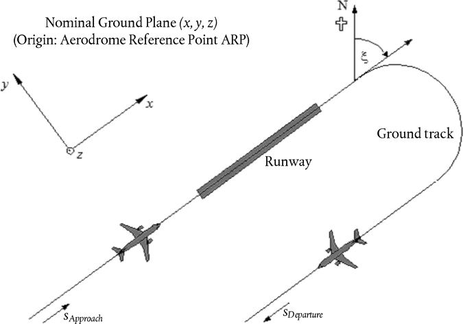
The ground-track fixed coordinate system U.K.
This coordinate is specific for each ground track and represents distance s measured along the track in the flight direction. For departure tracks s is measured from the start of roll, for approach tracks from the landing threshold. Thus s becomes negative in areas
behind the start of roll for departures and
before crossing the runway landing threshold for approaches.
Flight operational parameters such as height, speed and power setting are expressed as functions of s.
The aircraft coordinate system U.K.
The aircraft-fixed Cartesian coordinate system (x′,y′,z′) has its origin at the actual aircraft location. The axis-system is defined by the climb-angle γ, the flight direction ξ and the bank-angle ε (see Figure 2.7.c).

Accounting for topography U.K.
In cases where topography has to be taken into account (see Section 2.7.6), the aircraft height coordinate z has to be replaced by z′= z – zo (where zo is the z-coordinate of the observer location O) when estimating the propagation distance d. The geometry between aircraft and observer is shown in Figure 2.7.d. For the definitions of d and ℓ see Sections 2.7.14 to 2.7.19(10).
Figure 2.7.d
Ground elevation along (left) and lateral (right) to ground track
(The nominal ground plane z = 0 passes through the aerodrome reference point. O is the observer location.)

2.7.11. Ground Tracks U.K.
Backbone tracks U.K.
The backbone track defines the centre of the swathe of tracks followed by aircraft using a particular routeing. For the purposes of aircraft noise modelling it is defined either (i) by prescriptive operational data such as the instructions given to pilots in AIPs, or (ii) by statistical analysis of radar data as explained in Section 2.7.9 — when this is available and appropriate to the needs of the modelling study. Constructing the track from operational instructions is normally quite straightforward as these prescribe a sequence of legs which are either straight — defined by length and heading, or circular arcs defined by turn rate and change of heading; see Figure 2.7.e for an illustration.

Fitting a backbone track to radar data is more complex, firstly because actual turns are made at a varying rate and secondly because its line is obscured by the scatter of the data. As explained, formalised procedures have not yet been developed and it is common practice to match segments, straight and curved, to the average positions calculated from cross-sections of radar tracks at intervals along the route. Computer algorithms to perform this task are likely to be developed in future but, for the present, it is for the modeller to decide how to use available data to best advantage. A major factor is that the aircraft speed and turn radius dictate the angle of bank and, as will be seen in Section 2.7.19, non-symmetries of sound radiation around the flight path govern noise on the ground, as well as the position of the flight path itself.
Theoretically, seamless transition from straight flight to fixed radius turn would require an instantaneous application of bank angle ε, which is physically impossible. In reality it takes a finite time for the bank angle to reach the value required to maintain a specified speed and turn radius r, during which the turn radius tightens from infinity to r. For modelling purposes the radius transition can be disregarded and the bank angle assumed to increase steadily from zero (or other initial value) to ε at the start of the turn and to be the next value of ε at the end of the turn(11).
Track dispersion U.K.
Where possible, definitions of lateral dispersion and representative sub-tracks shall be based on relevant past experience from the study airport; normally via an analysis of radar data samples. The first step is to group the data by route. Departure tracks are characterised by substantial lateral dispersion which, for accurate modelling, has to be taken into account. Arrival routes normally coalesce into a very narrow swathe about the final approach path and it is usually sufficient to represent all arrivals by a single track. But if the approach swathes are wide within the region of the noise contours they might need to be represented by sub-tracks in the same way as departure routes.
It is common practice to treat the data for a single route as a sample from a single population; i.e. to be represented by one backbone track and one set of dispersed subtracks. However, if inspection indicates that the data for different categories of aircraft or operations differ significantly (e.g. should large and small aircraft have substantially different turn radii), further subdivision of the data into different swathes may be desirable. For each swathe, the lateral track dispersions are determined as a function of distance from the origin; movements then being apportioned between a backbone track and a suitable number of dispersed sub-tracks on the basis of the distribution statistics.
As it is normally unwise to disregard the effects of track dispersion, in the absence of measured swathe data a nominal lateral spread across and perpendicular to the backbone track shall be defined by a conventional distribution function. Calculated values of noise indices are not particularly sensitive to the precise shape of the lateral distribution: the Normal (Gaussian) Distribution provides an adequate description of many radar-measured swathes.
Typically a 7-point discrete approximation is used (i.e. representing the lateral dispersion by 6 subtracks equally spaced around the backbone track). The spacing of the subtracks depends on the standard deviation of the lateral dispersion function.
For normally distributed tracks with a standard deviation S, 98,8 % of the tracks are located within a corridor with boundaries located at ± 2,5 · S. Table 2.7.a gives the spacing of the six subtracks and the percentage of the total movements assigned to each. Appendix C gives values for other numbers of subtracks.
Table 2.7.a
Percentages of movements for a normal distribution function with standard deviation S for 7 subtracks (backbone track is subtrack 1)
| Subtrack number | Location of subtrack | Percentage of movements on subtrack |
|---|---|---|
| 7 | – 2,14 · S | 3 % |
| 5 | – 1,43 · S | 11 % |
| 3 | – 0,71 · S | 22 % |
| 1 | 0 | 28 % |
| 2 | 0,71 · S | 22 % |
| 4 | 1,43 · S | 11 % |
| 6 | 2,14 · S | 3 % |
The standard deviation S is a function of the coordinate s along the backbone-track. It can be specified — together with the description of the backbone-track — in the flight track data sheet shown in Appendix A3. In the absence of any indicators of the standard deviation — e.g. from radar data describing comparable flight tracks — the following values are recommended:
For tracks involving turns of less than 45 degrees:
S(s) = 0,055 · s – 150 for 2 700 m ≤ s ≤30 000 m (2.7.1) S(s) = 1 500 for s > 30 000 m For tracks involving turns of more than 45 degrees:
S(s) = 0,128 · s – 420 for 3 300 m ≤ s ≤ 15 000 m (2.7.2) S(s) = 1 500 m for s > 15 000 m
For practical reasons, S(s) is assumed to be zero between the start of roll and s = 2 700 m or s = 3 300 m depending on the amount of turn. Routes involving more than one turn shall be treated as per equation (2.7.2). For arrivals, lateral dispersion can be neglected within 6 000 m of touchdown.
2.7.12. Flight profiles U.K.
The flight profile is a description of the aircraft motion in the vertical plane above the ground track, in terms of its position, speed, bank angle and engine power setting. One of the most important tasks facing the model user is that of defining aircraft flight profiles that adequately meet the requirements of the modelling application — efficiently, without consuming excessive time and resources. Naturally, to achieve high accuracy, the profiles have to reflect closely the aircraft operations they are intended to represent. This requires reliable information on the atmospheric conditions, aircraft types and variants, operating weights and the operating procedures — the variations of thrust and flap settings and the trade-offs between changes of height and speed — all appropriately averaged over the time period(s) of interest. Often such detailed information are not available but this is not necessarily an obstacle; even if they are, the modeller has to exercise judgement to balance the accuracy and detail of the input information with the needs for, and uses of, the contour outputs.
The synthesis of flight profiles from ‘procedural steps’ obtained from the ANP database or from aircraft operators is described in Section 2.7.13 and Appendix B. That process, usually the only recourse open to the modeller when no radar data are available, yields both the flight path geometry and the associated speed and thrust variations. It would normally be assumed that all (alike) aircraft in a swathe, whether assigned to the backbone or the dispersed subtracks, follow the backbone track profile.
Beyond the ANP database, which provides default information on procedural steps, the aircraft operators are the best source of reliable information, i.e. the procedures they use and the typical weights flown. For individual flights, the ‘gold standard’ source is the aircraft flight data recorder (FDR) from which all relevant information can be obtained. But even if such data are available, the pre-processing task is formidable. Thus, and in keeping with the necessary modelling economies, the normal practical solution is to make educated assumptions about mean weights and operating procedures.
Caution must be exercised before adopting default procedural steps provided in the ANP database (customarily assumed when actual procedures are not known). These are standardised procedures that are widely followed but which may or may not be used by operators in particular cases. A major factor is the definition of take-off (and sometimes climb) engine thrust that can depend to an extent on prevailing circumstances. In particular, it is common practice to reduce thrust levels during departure (from maximum available) in order to extend engine life. Appendix B gives guidance on representing typical practice; this will generally produce more realistic contours than a full thrust assumption. However, if, for example, runways are short and/or average air temperatures are high, full thrust is likely to be a more realistic assumption.
When modelling actual scenarios, improved accuracy can be achieved by using radar data to supplement or replace this nominal information. Flight profiles can be determined from radar data in a similar way to the lateral backbone tracks — but only after segregating the traffic by aircraft type and variant and sometimes by weight or stage length (but not by dispersion) — to yield for each sub-group a mean profile of height and speed against ground distance travelled. Again, when merging with the ground tracks subsequently, this single profile is normally assigned to the backbone and subtracks alike.
Knowing the aircraft weight, the variation of speed and propulsive thrust can be calculated via step-by-step solution of the equations of motion. Before doing so it is helpful to pre-process the data to minimise the effects of radar errors which can make acceleration estimates unreliable. The first step in each case is to redefine the profile by fitting straight line segments to represent the relevant stages of flight; with each segment being appropriately classified; i.e. as a ground roll, constant speed climb or descent, thrust cutback, or acceleration/deceleration with or without flap change. The aircraft weight and atmospheric state are also required inputs.
Section 2.7.11 makes it clear that special provision has to be made to account for the lateral dispersion of flight tracks about the nominal or backbone routeings. Radar data samples are characterised by similar dispersions of flight paths in the vertical plane. However it is not usual practice to model vertical dispersion as an independent variable; it arises mainly due to differences in aircraft weights and operating procedures that are taken into account when pre-processing traffic input data.
2.7.13. Construction of flight path segments U.K.
Each flight path has to be defined by a set of segment coordinates (nodes) and flight parameters. The starting point is to determine the coordinates of the ground track segments. The flight profile is then calculated, remembering that for a given set of procedural steps, the profile depends on the ground track; e.g. at the same thrust and speed the aircraft climb rate is less in turns than in straight flight. Finally the 3-D flight path segments are constructed by merging the 2-D flight profile with the 2-D ground track(12).
Ground track U.K.
A ground track, whether a backbone track or a dispersed sub-track, is defined by a series of (x,y) coordinates in the ground plane (e.g. from radar information) or by a sequence of vectoring commands describing straight segments and circular arcs (turns of defined radius r and change of heading Δξ).
For segmentation modelling, an arc is represented by a sequence of straight segments fitted to sub-arcs. Although they do not appear explicitly in the ground-track segments, the banking of aircraft during turns influences their definition. Appendix B4 explains how to calculate bank angles during a steady turn but of course these are not actually applied or removed instantaneously. How to handle the transitions between straight and turning flight, or between one turn and an immediately sequential one, is not prescribed. As a rule, the details, which are left to the user (see Section 2.7.11), are likely to have a negligible effect on the final contours; the requirement is mainly to avoid sharp discontinuities at the ends of the turn and this can be achieved simply, for example, by inserting short transition segments over which the bank angle changes linearly with distance. Only in the special case that a particular turn is likely to have a dominating effect on the final contours would it be necessary to model the dynamics of the transition more realistically, to relate bank angle to particular aircraft types and to adopt appropriate roll rates. Here it is sufficient to state that the end sub-arcs Δξtrans in any turn are dictated by bank angle change requirements. The remainder of the arc with change of heading Δξ – 2 · Δξtrans degrees is divided into nsub sub-arcs according to the equation:
| nsub = int(1 + (Δξ – 2 · Δξtrans )/30) | (2.7.3) |
where int(x) is a function that returns the integer part of x. Then the change of heading Δξsub of each sub-arc is computed as
| Δξsub = (Δξ – 2 · Δξtrans )/nsub | (2.7.4) |
where nsub needs to be large enough to ensure that Δξsub ≤ 30 degrees. The segmentation of an arc (excluding the terminating transition sub-segments) is illustrated in Figure 2.7.f (13).
Figure 2.7.f
Construction of flight path segments dividing turn into segments of length Ds (upper view in horizontal plane, lower view in vertical plane)

Flight profile U.K.
The parameters describing each flight profile segment at the start (suffix 1) and end (suffix 2) of the segment are:
s 1, s 2
distance along the ground track,
z 1, z 2
aeroplane height,
V 1, V 2
groundspeed,
P 1, P 2
noise-related power parameter (matching that for which the NPD-curves are defined), and
ε1, ε2
bank angle.
To build a flight profile from a set of procedural steps (flight path synthesis), segments are constructed in sequence to achieve required conditions at the end points. The end-point parameters for each segment become the start-point parameters for the next segment. In any segment calculation the parameters are known at the start; required conditions at the end are specified by the procedural step. The steps themselves are defined either by the ANP defaults or by the user (e.g. from aircraft flight manuals). The end conditions are usually height and speed; the profile building task is to determine the track distance covered in reaching those conditions. The undefined parameters are determined via flight performance calculations described in Appendix B.
If the ground track is straight, the profile points and associated flight parameters can be determined independently of the ground track (bank angle is always zero). However ground tracks are rarely straight; they usually incorporate turns and, to achieve best results, these have to be accounted for when determining the 2-dimensional flight profile, where necessary splitting profile segments at ground track nodes to inject changes of bank angle. As a rule the length of the next segment is unknown at the outset and it is calculated provisionally assuming no change of bank angle. If the provisional segment is then found to span one or more ground track nodes, the first being at s, i.e. s1 < s < s2 , the segment is truncated at s, calculating the parameters there by interpolation (see below). These become the end-point parameters of the current segment and the start-point parameters of a new segment — which still has the same target end conditions. If there is no intervening ground track node the provisional segment is confirmed.
If the effects of turns on the flight profile are to be disregarded, the straight flight, single segment solution is adopted although the bank angle information is retained for subsequent use.
Whether or not turn effects are fully modelled, each 3-dimensional flight path is generated by merging its 2-dimensional flight profile with its 2-dimensional ground track. The result is a sequence of coordinate sets (x,y,z), each being either a node of the segmented ground track, a node of the flight profile or both, the profile points being accompanied by the corresponding values of height z, ground speed V, bank angle ε and engine power P. For a track point (x,y) which lies between the end points of a flight profile segment, the flight parameters are interpolated as follows:


Where
| f = (s – s1)/(s2 – s1) | (2.7.9) |
Note that whilst z and ε are assumed to vary linearly with distance, V and P are assumed to vary linearly with time (i.e. constant acceleration(14)).
When matching flight profile segments to radar data (flight path analysis) all end-point distances, heights, speeds and bank angles are determined directly from the data; only the power settings have to be calculated using the performance equations. As the ground track and flight profile coordinates can also be matched appropriately, this is usually quite straightforward.
Segmentation of the takeoff ground roll U.K.
When taking off, as an aircraft accelerates between the point of brake release (alternatively termed Start-of-Roll SOR) and the point of lift-off, speed changes dramatically over a distance of 1 500 to 2 500 m, from zero to between around 80 and 100 m/s.
The takeoff roll is thus divided into segments with variable lengths over each of which the aircraft speed changes by specific increment ΔV of no more than 10 m/s (about 20 kt). Although it actually varies during the takeoff roll, an assumption of constant acceleration is adequate for this purpose. In this case, for the takeoff phase, V1 is initial speed, V2 is the takeoff speed, nTO is the number of takeoff segment and sTO is the equivalent takeoff distance. For equivalent takeoff distance sTO (see Appendix B), start speed V1 and takeoff speed V2 the number nTO of segments for the ground roll is
| nTO = int(1 + (V2 – V1 )/10) | (2.7.10) |
and hence the change of velocity along a segment is
| ΔV = (V2 – V1)/nTO | (2.7.11) |
and the time Δt on each segment is (constant acceleration assumed)

The length sTO,k of segment k (1 ≤ k ≤ nTO) of the takeoff roll is then:

Example: U.K.
For a takeoff distance sTO = 1 600 m, V1 = 0 m/s and V2 = 75 m/s, this yields nTO = 8 segments with lengths ranging from 25 to 375 meters (see Figure 2.7.g):U.K.

Similarly to the speed changes, the aircraft thrust changes over each segment by a constant increment ΔP, calculated as
| ΔP = (PTO – Pinit)/nTO | (2.7.14) |
where PTO and Pinit respectively designate the aircraft thrust at the point of lift-off and the aircraft thrust at the start of takeoff roll.
The use of this constant thrust increment (instead of using the quadratic form (equation (2.7.8)) aims at being consistent with the linear relationship between thrust and speed in the case of jet-engine aircraft (eq. B-1).
Segmentation of the initial climb segment U.K.
During the initial climb segment the geometry is changing rapidly particularly with respect to observer locations to the side of the flight track, where beta angle will change rapidly as the aircraft climbs through this initial segment. Comparisons with very small segment calculations show that a single climb segment results in a poor approximation of noise to the side of the flight track for integrated metrics. Calculation accuracy is improved by sub-segmenting the first lift-off segment. The length of each segment and number is strongly influenced by lateral attenuation. Noting the expression of total lateral attenuation for aircraft with fuselage-mounted engines, it can be shown that for a limiting change in lateral attenuation of 1,5 dB per sub-segment, that the initial climb segment shall be sub-segmented based on the following set of height values:
z = {18,9, 41,5, 68,3, 102,1, 147,5, 214,9, 334,9, 609,6, 1 0289,6} metres, or
z = {62, 136, 224, 335, 484, 705, 1 099, 2 000, 4 231} feet
The above heights are implemented by identifying which height in the set above is closest to the original segment endpoint. The actual sub-segment heights would then be calculated using:
| z′i = z [zi/zN] (i = 1…N) | (2.7.15) |
where z is the original segment end height, zi is the ith member of the set of height values and zN is the closest upper bound to height z. This process results in the lateral attenuation change across each sub-segment remaining constant, producing more accurate contours, but without the expense of using very short segments.
Example: U.K.
If the original segment endpoint height is at z = 304,8 m, then from the set of height values, 214,9 < 304,8 < 334,9 and the closest upper bound is to z = 304,8 m is z7 = 334,9 m. The sub-segment endpoint heights are then computed by:U.K.
zi′ = 304,8 [zi/334,9] (i = 1..N)
Thus z1′ would be 17,2 m and z2′ would be 37,8 m, etc.
The speed and engine power values on the inserted points are interpolated using respectively equations (2.7.11) and (2.7.13)
Segmentation of airborne segments U.K.
After the segmented flight path has been derived according to the procedure described in Section 2.7.13 and the sub-segmenting described is applied, further segmentation adjustments may be necessary. These include
the removal of flight path points which are too close together and
the insertion of additional points when speed changes along segments are too long.
When adjacent points are within 10 metres of each other, and when the associated speeds and thrusts are the same, one of the points shall be eliminated.
For airborne segments where there is a significant speed change along a segment, this shall be subdivided as for the ground roll, i.e.

where V1 and V2 are the segment start and end speeds respectively. The corresponding sub-segment parameters are calculated in a similar manner as for the takeoff ground roll, using equations (2.7.11) to (2.7.13).
The landing ground roll U.K.
Although the landing ground roll is essentially a reversal of the takeoff ground roll, special account has to be taken of
reverse thrust which is sometimes applied to decelerate the aircraft and
aeroplanes leaving the runway after deceleration (aircraft that leave the runway no longer contribute to air noise as noise from taxiing is disregarded).
In contrast to the takeoff roll distance, which is derived from aircraft performance parameters, the stop distance sstop (i.e. the distance from touchdown to the point where the aircraft leaves the runway) is not purely aircraft specific. Although a minimum stop distance can be estimated from aircraft mass and performance (and available reverse thrust), the actual stop distance depends also on the location of the taxiways, on the traffic situation, and on airport-specific regulations on the use of reverse thrust.
The use of reverse thrust is not a standard procedure — it is only applied if the needed deceleration cannot be achieved by the use of the wheel brakes. (Reverse thrust can be exceptionally disturbing as a rapid change of engine power from idle to reverse settings produces a sudden burst of noise.)
However, most runways are used for departures as well as for landings so that reverse thrust has a very small effect on the noise contours since the total sound energy in the vicinity of the runway is dominated by the noise produced from takeoff operations. Reverse thrust contributions to contours may only be significant when runway use is limited to landing operations.
Physically, reverse thrust noise is a very complex process but because of its relatively minor significance to air noise contours it can be modelled simplistically — the rapid change in engine power being taken into account by suitable segmentation.
It is clear that modelling the landing ground roll is less straightforward than for takeoff roll noise. The following simplified modelling assumptions are recommended for general use, when no detailed information is available (see Figure 2.7.h).

The aeroplane touches down 300 meters beyond the landing threshold (which has the coordinate s = 0 along the approach ground track). The aircraft is then decelerated over a stop-distance sstop — aircraft specific values of which are given in the ANP database — from final approach speed Vfinal to 15 m/s. Because of the rapid changes in speed during this segment it shall be sub-segmented in the same manner as for the takeoff ground roll (or airborne segments with rapid speed changes), using equations (2.7.10) to (2.7.13).
The engine power changes from final approach power at touchdown to a reverse thrust power setting Prev over a distance 0,1 · sstop , then decreases to 10 % of the maximum available power over the remaining 90 percent of the stop distance. Up to the end of the runway (at s = – sRWY ) aircraft speed remains constant.
NPD curves for reverse thrust are not at present included in the ANP database, and it is therefore necessary to rely on the conventional curves for modelling this effect. Typically the reverse thrust power Prev is around 20 % of the full power setting and this is recommended when no operational information is available. However, at a given power setting, reverse thrust tends to generate significantly more noise than forward thrust and an increment ΔL shall be applied to the NPD-derived event level, increasing from zero to a value ΔLrev (5 dB is recommended provisionally(15)) along 0,1 · sstop and then falling linearly to zero along the remainder of the stop distance.
2.7.14. Noise calculation for a single event U.K.
The core of the modelling process, described here in full, is the calculation of the event noise level from the flight path information described in Sections 2.7.7 to 2.7.13.
2.7.15. Single event metrics U.K.
The sound generated by an aircraft movement at the observer location is expressed as a ‘single event sound (or noise) level’, a quantity which is an indicator of its impact on people. The received sound is measured in noise terms using a basic decibel scale L(t) which applies a frequency weighting (or filter) to mimic a characteristic of human hearing. The scale of most importance in aircraft noise contour modelling is A-weighted sound level, LA .
The metric most commonly used to encapsulate entire events is ‘single event sound (or noise) exposure levels’, LE , which account for all (or most of) the sound energy in the events. Making provisions for the time integration that this involves gives rise to the main complexities of segmentation (or simulation) modelling. Simpler to model is an alternative metric Lmax which is the maximum instantaneous level occurring during the event; however it is LE which is the basic building block of most modern aircraft noise indices and practical models can in future be expected to embody both Lmax and LE . Either metric can be measured on different scales of noise; in this document only A-weighted sound level is considered. Symbolically, the scale is usually indicated by extending the metric suffix, i.e. LAE , LAmax .
The single event sound (or noise) exposure level is expressed exactly as

where t 0 denotes a reference time. The integration interval [t1,t2] is chosen to ensure that (nearly) all significant sound in the event is encompassed. Very often, the limits t1 and t2 are chosen to span the period for which the level L(t) is within 10 dB of Lmax . This period is known as the ‘10-dB down’ time. Sound (noise) exposure levels tabulated in the ANP database are 10-dB down values(16).
For aircraft noise contour modelling, the main application of equation (2.7.17) is the standard metric Sound Exposure Level LAE (acronym SEL):
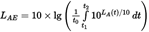
The exposure level equations above can be used to determine event levels when the entire time history of L(t) is known. Within the recommended noise modelling methodology such time histories are not defined; event exposure levels are calculated by summing segment values, partial event levels each of which defines the contribution from a single, finite segment of the flight path.
2.7.16. Determination of event levels from NPD-data U.K.
The principal source of aircraft noise data is the international Aircraft Noise and Performance (ANP) database. This tabulates Lmax and LE as functions of propagation distance d — for specific aircraft types, variants, flight configurations (approach, departure, flap settings), and power settings P. They relate to steady flight at specific reference speeds Vref along a notionally infinite, straight flight path(17).
How values of the independent variables P and d are specified is described later. In a single look-up, with input values P and d, the output values required are the baseline levels Lmax(P,d) and/or LE∞(P,d) (applicable to an infinite flight path). Unless values happen to be tabulated for P and/or d exactly, it will generally be necessary to estimate the required event noise level(s) by interpolation. A linear interpolation is used between tabulated power-settings, whereas a logarithmic interpolation is used between tabulated distances (see Figure 2.7.i).

If Pi and Pi + 1 are engine power values for which noise level versus distance data are tabulated, the noise level L(P) at a given distance for intermediate power P, between Pi and Pi + 1 , is given by:

If, at any power setting, di and di + 1 are distances for which noise data are tabulated, the noise level L(d) for an intermediate distance d, between di and di + 1 is given by

By using equations (2.7.19) and (2.7.20), a noise level L(P,d) can be obtained for any power setting P and any distance d that is within the envelope of the NPD data base.
For distances d that lie outside the NPD envelope, equation (2.7.20) is used to extrapolate from the last two values, i.e. inwards from L(d1) and L(d2) or outwards from L(dI – 1) and L(dI) where I is the total number of NPD points on the curve. Thus


As, at short distances d, noise levels increase very rapidly with decreasing propagation distance, it is recommended that a lower limit of 30 m be imposed on d, i.e. d = max(d, 30 m).
Impedance adjustment of standard NPD data U.K.
The NPD data provided in the ANP database are normalised to specific atmospheric conditions (temperature of 25 °C and pressure of 101,325 kPa). Before applying the interpolation/extrapolation method previously described, an acoustic impedance adjustment shall be applied to these standard NPD data.
Acoustic impedance is related to the propagation of sound waves in an acoustic medium, and is defined as the product of the density of air and the speed of sound. For a given sound intensity (power per unit area) perceived at a specific distance from the source, the associated sound pressure (used to define SEL and LAmax metrics) depends on the acoustic impedance of the air at the measurement location. It is a function of temperature, atmospheric pressure (and indirectly altitude). There is therefore a need to adjust the standard NPD data of the ANP database to account for the actual temperature and pressure conditions at the receiver point, which are generally different from the normalised conditions of the ANP data.
The impedance adjustment to be applied to the standard NPD levels is expressed as follows:

where:
ΔImpedance
Impedance adjustment for the actual atmospheric conditions at the receiver point (dB)
ρ · c
Acoustic impedance (newton · seconds/m3) of the air at the receiver point (409,81 being the air impedance associated to the reference atmospheric conditions of the NPD data in the ANP database).
Impedance ρ · c is calculated as follows:
 | (2.7.24) |
δ
p/po , the ratio of the ambient air pressure at the observer altitude to the standard air pressure at mean sea level: po = 101,325 kPa (or 1013,25 mb)
θ
(T + 273,15)/(T0 + 273,15) the ratio of the air temperature at the observer altitude to the standard air temperature at mean sea level: T0 = 15,0 °C
The acoustic impedance adjustment is usually less than a few tenths of one dB. In particular, it should be noted that under the standard atmospheric conditions (po = 101,325 kPa and T0 = 15,0 °C), the impedance adjustment is less than 0,1 dB (0,074 dB). However, when there is a significant variation in temperature and atmospheric pressure relative to the reference atmospheric conditions of the NPD data, the adjustment can be more substantial.
2.7.17. General expressions U.K.
Segment event level Lseg U.K.
The segment values are determined by applying adjustments to the baseline (infinite path) values read from the NPD data. The maximum noise level from one flight path segment Lmax,seg can be expressed in general as
 | (2.7.25) |
and the contribution from one flight path segment to LE as
 | (2.7.26) |
The ‘correction terms’ in equations (2.7.25) and (2.7.26) — which are described in detail in Section 2.7.19 — account for the following effects:
Δ V
Duration correction: the NPD data relate to a reference flight speed. This adjusts exposure levels to non-reference speeds. (It is not applied to Lmax,seg .)
Δ I (φ)
Installation effect: describes a variation in lateral directivity due to shielding, refraction and reflection caused by the airframe, engines and surrounding flow fields.
Λ(β,ℓ)
Lateral attenuation: significant for sound propagating at low angles to the ground, this accounts for the interaction between direct and reflected sound waves (ground effect) and for the effects of atmospheric non-uniformities (primarily caused by the ground) that refract sound waves as they travel towards the observer to the side of the flight path.
Δ F
Finite segment correction (noise fraction): accounts for the finite length of the segment which obviously contributes less noise exposure than an infinite one. It is only applied to exposure metrics.
If the segment is part of the take-off or landing ground roll and the observer is located behind the segment under consideration, special steps are taken to represent the pronounced directionality of jet engine noise that is observed behind an aircraft about to takeoff. These special steps result in particular in the use of a particular form of the noise for the exposure level:
 | (2.7.27) |
 | (2.7.28) |
Δ′ F
Particular form of the Segment correction
Δ SOR
Directivity correction: accounts for the pronounced directionality of jet engine noise behind the ground roll segment
The specific treatment of ground roll segments is described in Section 2.7.19.
Sections below describe the calculation of segment noise levels.
Event noise level L of an aircraft movement U.K.
Maximum level Lmax is simply the greatest of the segment values Lmax,seg (see equations (2.7.25) and (2.7.27))
| Lmax = max(Lmax,seg ) | (2.7.29) |
where each segment value is determined from the aircraft NPD data for power P and distance d. These parameters and the modifier terms ΔI (φ) and Λ(β,ℓ) are explained below.
Exposure level LE is calculated as the decibel sum of the contributions LE,seg from each noise-significant segment of its flight path; i.e.

The summation proceeds step by step through the flight path segments.
The remainder of this chapter is concerned with the determination of the segment noise levels Lmax,seg and LE,seg .
2.7.18. Flight path segment parameters U.K.
The power P, and distance d, for which the baseline levels Lmax,seg(P,d) and LE∞(P,d) are interpolated from the NPD tables, are determined from geometric and operational parameters that define the segment. How this is done is explained below with the aid of illustrations of the plane containing the segment and the observer.
Geometric parameters U.K.
Figures 2.7.j to 2.7.l show the source-receiver geometries when the observer O is (a) behind, (b) alongside and (c) ahead of the segment S1S2 where the flight direction is from S1 to S2 . In these diagrams
O
is the observer location
S1 , S2
are the start and end of the segment
Sp
is the point of perpendicular closest approach to the observer on the segment or its extension
d 1, d 2
are the distances between start, end of segment and observer
ds
is the shortest distance between observer and segment
dp
is the perpendicular distance between observer and extended segment (minimum slant range)
λ
is the length of flight path segment
q
is the distance from S1 to Sp (negative if the observer position is behind the segment)
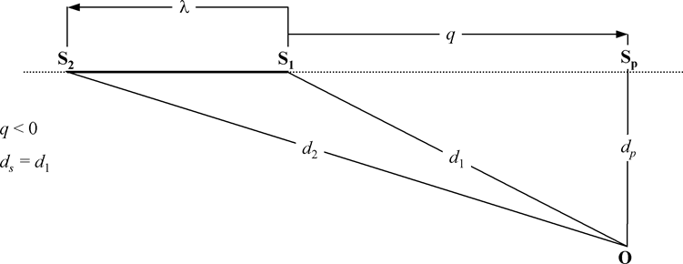
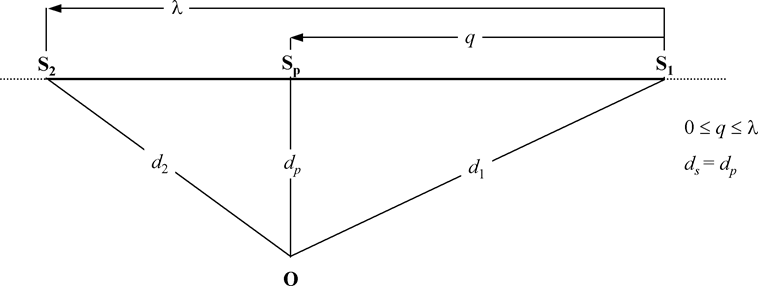

The flight path segment is represented by a bold, solid line. The dotted line represents the flight path extension which stretches to infinity in both directions. For airborne segments, when the event metric is an exposure level LE , the NPD distance parameter d is the distance dp between Sp and the observer, called the minimum slant range (i.e. the perpendicular distance from the observer to the segment or its extension, in other words to the (hypothetical) infinite flight path of which the segment is considered to be part).
However, for exposure level metrics where observer locations are behind the ground segments during the takeoff roll and locations ahead of ground segments during the landing roll, the NPD distance parameter d becomes the distance ds , the shortest distance from the observer to the segment (i.e. the same as for maximum level metrics).
For maximum level metrics, the NPD distance parameter d is ds , the shortest distance from the observer to the segment.
Segment power P U.K.
The tabulated NPD data describe the noise of an aircraft in steady straight flight on an infinite flight path, i.e. at constant engine power P. The recommended methodology breaks actual flight paths, along which speed and direction vary, into a number of finite segments, each of which is then taken to be part of a uniform, infinite flight path for which the NPD data are valid. But the methodology provides for changes of power along the length of a segment; it is taken to change linearly with distance from P1 at its start to P2 at its end. It is therefore necessary to define an equivalent steady segment value P. This is taken to be the value at the point on the segment that is closest to the observer. If the observer is alongside the segment (Figure 2.7.k) it is obtained by interpolation as given by equation (2.7.8) between the end values, i.e.

If the observer is behind or ahead of the segment, it is that at the nearest end point, P1 or P2 .
2.7.19. Segment Event level correction terms U.K.
The NPD data define noise event levels as a function of distance perpendicularly beneath an idealised straight level path of infinite length along which the aircraft flies with steady power at a fixed reference speed(18). The event level interpolated from the NPD table for a specific power setting and slant distance is thus described as a baseline level. It applies to an infinite flight path and has to be corrected to account for the effects of (1) non-reference speed, (2) engine installation effects (lateral directivity), (3) lateral attenuation, (4) finite segment length and (5) longitudinal directivity behind start of roll on takeoff — see equations (2.7.25) and (2.7.26).
The duration correction DV (Exposure levels LE only) U.K.
This correction(19) accounts for a change in exposure levels if the actual segment groundspeed is different to the aircraft reference speed Vref to which the basic NPD-data relate. Like engine power, speed varies along the segment (groundspeed varies from V1 to V2) and it is necessary to define an equivalent segment speed Vseg remembering that the segment is inclined to the ground; i.e.
| Vseg = V/cosγ | (2.7.32) |
where here V is an equivalent segment groundspeed (for information, see equation B-22 which expresses V in terms of calibrated airspeed, Vc and

For airborne segments, V is taken to be the groundspeed at the closest point of approach S — interpolated between the segment end-point values assuming it varies linearly with time; i.e. if the observer is alongside the segment:

If the observer is behind or ahead of the segment, it is that at the nearest end point, V1 or V2 .
For runway segments (parts of the take-off or landing ground rolls for which γ = 0) Vseg is taken to be simply the average of the segment start and end speeds; i.e.
| Vseg = (V1 + V2 )/2 | (2.7.35) |
In either case the additive duration correction is then
| ΔV = 10 · lg(Vref/Vseg ) | (2.7.36) |
Sound propagation geometry U.K.
Figure 2.7.l shows the basic geometry in the plane normal to the aircraft flight path. The ground line is the intersection of the normal plane and the level ground plane. (If the flight path is level the ground line is an end view of the ground plane.) The aircraft is banked at angle ε measured counter-clockwise about its roll axis (i.e. starboard wing up). It is therefore positive for left turns and negative for right turns.

The elevation angle β (between 0 and 90°) between the direct sound propagation path and the level ground line(20) determines, together with the flight path inclination and the lateral displacement ℓ of the observer from the ground track, the lateral attenuation.
The depression angle φ between the wing plane and the propagation path, determines the engine installation effects. With respect to the convention for the bank angle φ = β ± ε with the sign positive for observers to starboard (right) and negative for observers to port (left).
Engine installation correction ΔI U.K.
An aircraft in flight is a complex sound source. Not only are the engine (and airframe) sources complex in origin, but the airframe configuration, particularly the location of the engines, influences the noise radiation patterns through the processes of reflection, refraction and scattering by the solid surfaces and aerodynamic flow fields. This results in a non-uniform directionality of sound radiated laterally about the roll axis of the aircraft, referred to here as lateral directivity.
There are significant differences in lateral directivity between aircraft with fuselage-mounted and underwing-mounted engines and these are allowed for in the following expression:

where Δ I (φ) is the correction, in dB, at depression angle φ (see Figure 2.7.m) and
| a = 0,00384, | b = 0,0621, | c = 0,8786 | for wing-mounted engines and |
| a = 0,1225, | b = 0,3290, | c = 1 | for fuselage-mounted engines. |
For propeller aircraft directivity variations are negligible and for these it may be assumed that
| ΔI (φ) = 0 | (2.7.38) |
Figure 2.7.n shows the variation of Δ I (φ) about the aircraft roll axis for the three engine installations. These empirical relationships have been derived by the SAE from experimental measurements made mainly beneath the wing. Until above-wing data have been analysed it is recommended that, for negative φ, Δ I (φ) = Δ I(0) for all installations.

It is assumed that Δ I (φ) is two-dimensional; i.e. it does not depend on any other parameter — and in particular that it does not vary with the longitudinal distance of the observer from the aircraft. This means that the elevation angle β for Δ I (φ) is defined as β = tan–1(z/ℓ). This is for modelling convenience until there is a better understanding of the mechanisms; in reality, installation effects are bound to be substantially three-dimensional. Despite that, a two-dimensional model is justified by the fact that event levels tend to be dominated by noise radiated sideways from the nearest segment.
Lateral attenuation Λ(β,ℓ) (infinite flight path) U.K.
Tabulated NPD event levels relate to steady level flight and are generally based on measurements made 1,2 m over soft level ground beneath the aircraft; the distance parameter is effectively height above the surface. Any effect of the surface on event noise levels beneath the aircraft, that might cause the tabulated levels to differ from free-field values(21), is assumed to be inherent in the data (i.e. in the shape of the level vs. distance relationships).
To the side of the flight path, the distance parameter is the minimum slant distance — the length of the normal from the receiver to the flight path. At any lateral position the noise level will generally be less than at the same distance immediately below the aircraft. Apart from lateral directivity or ‘installation effects’ described above is due to an excess lateral attenuation which causes the sound level to fall more rapidly with distance than indicated by the NPD curves. A previous, widely used method for modelling lateral propagation of aircraft noise was developed by the Society of Automotive Engineers (SAE) in AIR-1751 and the algorithms described below are based on improvements SAE now recommends AIR-5662. Lateral attenuation is a reflection effect, due to interference between directly radiated sound and that which reflects from the surface. It depends on the nature of the surface and can cause significant reductions in observed sound levels at low elevation angles. It is also very strongly affected by sound refraction, steady and unsteady, caused by wind and temperature gradients and turbulence which are themselves attributable to the presence of the surface(22). The mechanism of surface reflection is well understood and, for uniform atmospheric and surface conditions, it can be described theoretically with some precision. However, atmospheric and surface non-uniformities — which are not amenable to simple theoretical analysis — have a profound effect on the reflection effect, tending to ‘spread’ it to higher elevation angles; thus the theory is of limited applicability. SAE work to develop a better understanding of surface effects is continuing and this is expected to lead to better models. Until these are developed, the following methodology, described in AIR-5662, is recommended for calculating lateral attenuation. It is confined to the case of sound propagation over soft level ground which is appropriate for the great majority of civil airports. Adjustments to account for the effects of a hard ground surface (or, acoustically equivalent, water) are still under development.
The methodology is built on the substantial body of experimental data on sound propagation from aircraft with fuselage-mounted engines in straight (non-turning), steady, level flight reported originally in AIR-1751. Making the assumption that, for level flight, air-to-ground attenuation depends on (i) elevation angle β measured in the vertical plane and (ii) lateral displacement from the aircraft ground track ℓ, the data were analysed to obtain an empirical function for the total lateral adjustment Λ T (β,ℓ) (= lateral event level minus the level at the same distance beneath the aircraft).
As the term Λ T (β,ℓ) accounted for lateral directivity as well as lateral attenuation, the latter can be extracted by subtraction. Describing lateral directivity by equation (2.7.37), with the fuselage-mount coefficients and with φ replaced by β (appropriate to non-turning flight), the lateral attenuation becomes:
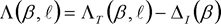 | (2.7.39) |
where β and ℓ are measured as depicted in Figure 2.7.m in a plane normal to the infinite flight path which, for level flight, is also vertical.
Although Λ(β,ℓ) could be calculated directly using equation (2.7.39) with Λ T (β,ℓ) taken from AIR-1751, a more efficient relationship is recommended. This is the following empirical approximation adapted from AIR-5662:
 | (2.7.40) |
where Γ(ℓ) is a distance factor given by
 | for 0 ≤ ℓ ≤ 914 m | (2.7.41) |
 | for ℓ > 914 m | (2.7.42) |
and Λ(β) is long-range air-to-ground lateral attenuation given by
| Λ(β) = 1,137 – 0,0229β + 9,72 · exp(– 0,142β) | for 0° ≤ β ≤ 50° | (2.7.43) |
| Λ(β) = 0 | for 50° ≤ β ≤ 90° | (2.7.44) |
The expression for lateral attenuation Λ(β,ℓ), equation (2.7.40), which is assumed to hold good for all aircraft, propeller aircraft as well as fuselage-mount and wing-mount jets, is shown graphically in Figure 2.7.o.
Under certain circumstances (with terrain), it is possible for β to be less than zero. In such cases it is recommended that Λ(β) = 10,57.

Finite segment lateral attenuation U.K.
Equations (2.7.41) to (2.7.44) describe the lateral attenuation Λ(β,ℓ) of sound arriving at the observer from an aeroplane in steady flight along an infinite, level flight path. When applying them to finite path segments that are not level, the attenuation has to be calculated for an equivalent level path — as the closest point on a simple extension of the inclined segment (that passes through the ground surface at some point) generally does not yield an appropriate elevation angle β.
The determination of lateral attenuation for finite segments differs markedly for Lmax and LE metrics. Segment maximum levels Lmax are determined from NPD data as a function of propagation distance d from the nearest point on the segment; no corrections are required to account for the dimensions of the segment. Likewise, lateral attenuation of Lmax is assumed to depend only on the elevation angle of, and ground distance to, the same point. Thus only the coordinates of that point are required. But for LE , the process is more complicated.
The baseline event level LE(P,d) that is determined from the NPD data, even though for finite segment parameters, applies nevertheless to an infinite flight path. The event exposure level from a segment, LE,seg , is of course less than the baseline level — by the amount of the finite segment correction defined later in Section 2.7.19. That correction, a function of the geometry of triangles OS1S2 in Figures 2.7.j to 2.7.l, defines what proportion of the total infinite path noise energy received at O comes from the segment; the same correction applies, whether or not there is any lateral attenuation. But any lateral attenuation shall be calculated for the infinite flight path, i.e. as a function of its displacement and elevation, not those of the finite segment.
Adding the corrections Δ V and Δ I , and subtracting lateral attenuation Λ(β,ℓ) from the NPD baseline level gives the adjusted event noise level for equivalent steady level flight on an adjacent, infinite straight path. But the actual flight path segments being modelled, those that affect the noise contours, are rarely level; aircraft are usually climbing or descending.
Figure 2.7.p illustrates a departure segment S1S2 — the aircraft is climbing at an angle γ — but the considerations remain very similar for an arrival. The remainder of the ‘real’ flight path is not shown; suffice it to state that S1S2 represents just a part of the whole path (which in general will be curved). In this case, the observer O is alongside, and to the left of, the segment. The aircraft is banked (anti-clockwise about the flight path) at an angle ε to the lateral horizontal axis. The depression angle φ from the wing plane, of which the installation effect Δ I is a function (equation (2.7.39)), lies in the plane normal to the flight path in which ε is defined. Thus φ = β – ε where β = tan–1(h/ℓ) and ℓ is the perpendicular distance OR from the observer to the ground track; i.e. the lateral displacement of the observer(23). The aeroplane's closest point of approach to the observer, S, is defined by the perpendicular OS, of length (slant distance) dp . The triangle OS1S2 accords with Figure 2.7.k, the geometry for calculating the segment correction Δ F .
To calculate the lateral attenuation using equation (2.7.40) (where β is measured in a vertical plane), an equivalent level flight path is defined in the vertical plane through S1S2 and with the same perpendicular slant distance dp from the observer. This is visualised by rotating the triangle ORS, and its attached flight path about OR (see Figure 2.7.p) through angle γ thus forming the triangle ORS′. The elevation angle of this equivalent level path (now in a vertical plane) is β = tan–1(h/ℓ) (ℓ remains unchanged). In this case, observer alongside, the lateral attenuation Λ(β,ℓ) is the same for LE and Lmax metrics.
Figure 2.7.q illustrates the situation when the observer point O lies behind the finite segment, not alongside. Here the segment is observed as a more distant part of an infinite path; a perpendicular can only be drawn to point Sp on its extension. The triangle OS1S2 accords with Figure 2.7.j which defines the segment correction Δ F . But in this case the parameters for lateral directivity and attenuation are less obvious.

Remembering that, as conceived for modelling purposes, lateral directivity (installation effect) is two-dimensional, the defining depression angle φ is still measured laterally from the aircraft wing plane. (The baseline event level is still that generated by the aircraft traversing the infinite flight path represented by the extended segment.) Thus the depression angle is determined at the closest point of approach, i.e. φ = βp - ε where βp is angle SpOC.
For maximum level metrics, the NPD distance parameter is taken as the shortest distance to the segment, i.e. d = d 1. For exposure level metrics, it is the shortest distance dp from O to Sp on the extended flight path; i.e. the level interpolated from the NPD table is LE∞ (P 1, dp ).
The geometrical parameters for lateral attenuation also differ for maximum and exposure level calculations. For maximum level metrics the adjustment L(β,ℓ) is given by equation (2.7.40) with β = β 1 = sin–1(z1/d1 ) and 
When calculating the lateral attenuation for airborne segments only and exposure level metrics, ℓ remains the shortest lateral displacement from the segment extension (OC). But to define an appropriate value of β it is again necessary to visualise an (infinite) equivalent level flight path of which the segment can be considered part. This is drawn through S1′, height h above the surface, where h is equal to the length of RS1 the perpendicular from the ground track to the segment. This is equivalent to rotating the actual extended flight path through angle γ about point R (see Figure 2.7.q). Insofar as R is on the perpendicular to S1 , the point on the segment that is closest to O, the construction of the equivalent level path is the same as when O is alongside the segment.
The closest point of approach of the equivalent level path to the observer O is at S′, slant distance d, so that the triangle OCS′ so formed in the vertical plane then defines the elevation angle β = cos–1(ℓ/d). Although this transformation might seem rather convoluted, it should be noted that the basic source geometry (defined by d1 , d2 and φ) remains untouched, the sound travelling from the segment towards the observer is simply what it would be if the entire flight along the infinitely extended inclined segment (of which for modelling purposes the segment forms part) were at constant speed V and power P1 . The lateral attenuation of sound from the segment received by the observer, on the other hand, is related not to βp , the elevation angle of the extended path, but to β, that of the equivalent level path.
The case of an observer ahead of the segment is not described separately; it is evident that this is essentially the same as the case of the observer behind.
However, for exposure level metrics where observer locations are behind ground segments during the takeoff roll and locations ahead of ground segments during the landing roll, the value of β becomes the same as that for maximum level metrics, i.e. β = β1 = sin–1(z1/d1 ) and 
The finite segment correction ΔF (Exposure levels LE only) U.K.
The adjusted baseline noise exposure level relates to an aircraft in continuous, straight, steady level flight (albeit with a bank angle ε that is inconsistent with straight flight). Applying the (negative) finite segment correction ΔF = 10 · lg(F), where F is the energy fraction, further adjusts the level to what it would be if the aircraft traversed the finite segment only (or were completely silent for the remainder of the infinite flight path).
The energy fraction term accounts for the pronounced longitudinal directivity of aircraft noise and the angle subtended by the segment at the observer position. Although the processes that cause the directionality are very complex, studies have shown that the resulting contours are quite insensitive to the precise directional characteristics assumed. The expression for Δ F below is based on a fourth-power 90-degree dipole model of sound radiation. It is assumed to be unaffected by lateral directivity and attenuation. How this correction is derived is described in detail in Appendix E.
The energy fraction F is a function of the ‘view’ triangle OS1S2 defined in Figures 2.7.j to 2.7.l such that:

with


where dλ is known as the ‘scaled distance’ (see Appendix E). Note that Lmax(P, dp) is the maximum level, from NPD data, for perpendicular distance dp , NOT the segment Lmax .
It is advised to apply a lower limit of – 150 dB to Δ F .
In the particular case of observer locations behind every takeoff ground-roll segment and every landing ground-roll segment, a reduced form of the noise fraction expressed in equation (2.7.45) is used, which corresponds to the specific case of q = 0. This is computed using

where α2 = λ/dλ and ΔSOR is the start-of-roll directivity function defined by equations (2.7.51) and (2.7.52).
The rationale for using this particular form of noise fraction is further explained in the section below, as part of the start-of-roll directivity application method.
Specific Treatments of Ground-roll Segments, including the start-of-roll directivity function Δ SOR U.K.
In the case of ground roll segments, both for takeoff and landing, specific treatments are applied, which are described below.
The start-of-roll directivity function Δ SOR U.K.
The noise of jet aircraft — especially those equipped with lower by-pass ratio engines — exhibits a lobed radiation pattern in the rearward arc, which is characteristic of jet exhaust noise. This pattern is the more pronounced the higher the jet velocity and the lower the aircraft speed. This is of special significance for observer locations behind the start of roll, where both conditions are fulfilled. This effect is taken into account by a directivity function Δ SOR .
The function Δ SOR has been derived from several noise measurement campaigns using microphones adequately positioned behind and on the side of the SOR of departing jet aircraft.
Figure 2.7.r shows the relevant geometry. The azimuth angle ψ between the aircraft longitudinal axis and the vector to the observer is defined by

The relative distance q is negative (see Figure 2.7.j) so that ψ ranges from 0° in the direction of the aircraft forward heading to 180° in the reverse direction.

The function Δ SOR represents the variation of the overall noise emanating from the takeoff ground roll measured behind the start of roll, relatively to the overall noise from takeoff ground roll measured on the side of the SOR, at the same distance:
| LTGR(dSOR,ψ) = LTGR(dSOR,90°) + ΔSOR(dSOR,ψ) | (2.7.48) |
where LTGR (dSOR ,90°) is the overall takeoff ground roll noise level generated by all takeoff ground roll segments at the point distance dSOR to the side of the SOR. At distances dSOR less than a normalising distance dSOR,0 , the SOR directivity function is given by


If the distance dSOR exceeds the normalising distance dSOR,0 , the directivity correction is multiplied by a correction factor to account for the fact that the directivity becomes less pronounced for greater distances from the aircraft; i.e.

The normalising distance dSOR,0 equals 762 m (2 500 ft).
Treatment of receivers located behind each takeoff and landing ground-roll segment U.K.
The Δ SOR function described above mostly captures the pronounced directivity effect of the initial portion of the takeoff roll at locations behind the SOR (because it is the closest to the receivers, with the highest jet velocity to aircraft speed ratio). However, the use of the hence established Δ SOR is ‘generalised’ to positions behind each individual ground roll segment — both takeoff and landing —, so not only behind the Start-of-Roll point (in the case of takeoff).
The parameters dS and ψ are calculated relative to the start of each individual ground roll segment.
The event level Lseg for a location behind a given takeoff or landing ground-roll segment is calculated to comply with the formalism of the Δ SOR function: it is essentially calculated for the reference point located on the side of the start point of the segment, at the same distance dS as the actual point, and is further adjusted with Δ SOR to obtain the event level at the actual point.
This means that the different correction terms in the equations below shall use the geometric parameters corresponding to this reference point located on the side of the start point:
| Lmax,seg = Lmax(P,d = ds) + ΔI(φ) – Λ(β,l = ds) + ΔSOR | (2.7.53) |
| LE,seg = LE,∞(P,d = ds) + ΔV + ΔI(φ) – Λ(β,l = ds) + Δ′F + ΔSOR | (2.7.54) |
where Δ′ F is the reduced form of the noise fraction expressed in equation (2.7.46) for the case of q = 0 (as the reference point is located on the side of the start point) and remembering that dλ shall be calculated using dS (and not dp ):

2.7.20. Event noise level L of a general-aviation aircraft movement U.K.
The method described in Section 2.7.19 is applicable to propeller-engined general-aviation aircraft when they are treated as propeller aircraft with regard to engine installation effects.
The ANP database includes entries for several general aviation aircraft. Whilst these are often the most common general-aviation aircraft operating, there may be occasions when it is appropriate to use additional data.
Where the specific general aviation aircraft are either not known or not in the ANP database, it is recommended to use the more generic aircraft data, GASEPF and GASEPV respectively. These data sets represent a small single-engined general aviation aircraft with fixed-pitch and variable-pitch propellers respectively. Tables of entries are presented in Annex I (Tables I-11 I-17)
2.7.21. Method for the Calculation of Helicopter Noise U.K.
For the calculation of helicopter noise, the same calculation method used for fixed-wing aircraft (outlined in Section 2.7.14) may be used, provided helicopters are treated as propeller aircraft and engine-installation effects, associated with jet aircraft are not applied. Tables of entries for two different data sets are presented in Annex I (Tables I-18 I-27).
2.7.22. Noise associated with Engine Testing (Run-Up) Operations, taxiing and auxiliary power units U.K.
In such cases where it is considered that noise associated with engine testing and auxiliary power-units are to be modelled, these are modelled according to the chapter on industrial noise. Although it is normally not the case, noise from aircraft engine tests (sometimes referred to as ‘engine run-ups’) at airports can make a contribution to noise impacts. Usually carried out for engineering purposes to check engine performance, aircraft are safely positioned away from buildings, aircraft, vehicular and/or personnel movements to avoid any jet-blast related damage.
For additional safety and noise control reasons, airports, particularly those with maintenance facilities that can lead to frequent engine tests, can install so-called ‘noise pens’, 3-sided baffled enclosures specially designed to deflect and dissipate jet blast and noise. Investigating the noise impact of such facilities, which can be further attenuated and reduced by the use of additional earth bunds or substantial noise barrier fencing, is best accomplished by treating the noise pen as a source of industrial noise and using an appropriate noise and sound propagation model.
2.7.23. Calculation of cumulative levels U.K.
Sections 2.7.14 to 2.7.19 describe the calculation of the event sound noise level of a single aircraft movement at a single observer location. The total noise exposure at that location is calculated by accumulating the event levels of all noise-significant aircraft movements, i.e. all movements, inbound or outbound, that influence the cumulative level.
2.7.24. Weighted equivalent sound levels U.K.
Time-weighted equivalent sound levels, which account for all significant aircraft sound energy received, shall be expressed in a generic manner by the formula

The summation is performed over all N noise events during the time interval T 0 to which the noise index applies. LE,i is the single event noise exposure level of the i-th noise event. gi is a time-of-day dependent weighting factor (usually defined for day, evening and night periods). Effectively gi is a multiplier for the number of flights occurring during the specific periods. The constant C can have different meanings (normalising constant, seasonal adjustment etc.).
Using the relationship

where Δi is the decibel weighting for the i-th period, equation (2.7.56) can be rewritten as

i.e. the time-of-day weighting is expressed by an additive level offset.
2.7.25. The weighted number of operations U.K.
The cumulative noise level is estimated by summing the contributions from all different types or categories of aircraft using the different flight routes which comprise the airport scenario.
To describe this summation process the following subscripts are introduced:
i
index for aircraft type or category
j
index for flight track or subtrack (if subtracks are defined)
k
index for flight track segment
Many noise indices — especially equivalent sound levels — include time-of-day weighting factors gi in their definition (equations (2.7.56) and (2.7.57)).
The summation process can be simplified by introducing a ‘weighted number of operations’
| Mij = (gday · Nij,day + gevening · Nij,evening + gnight · Nij,night ) | (2.7.58) |
The values Nij represent the numbers of operations of aircraft type/category i on track (or subtrack) j during the day, evening and night period respectively(24).
From equation (2.7.57) the (generic) cumulative equivalent sound level Leq at the observation point (x,y) is

T 0 is the reference time period. It depends on — as well as the weighting factors gi — the specific definition of the weighted index used (e.g. LDEN ). LE,ijk is the single event noise level contribution from segment k of track or subtrack j for an operation of aircraft of category i. The estimation of LE,ijk is described in detail in Sections 2.7.14 to 2.7.19.
2.7.26. Standard grid calculation and refinement U.K.
When noise contours are obtained by interpolation between index values at rectangularly spaced grid points, their accuracy depends on the choice of the grid spacing (or mesh size) Δ G , especially within cells where large gradients in the spatial distribution of the index cause tight curvature of the contours (see Figure 2.7.s). Interpolation errors are reduced by narrowing the grid spacing, but as this increases the number of grid points, the computation time is increased. Optimising a regular grid mesh involves balancing modelling accuracy and run time.

A marked improvement in computing efficiency that delivers more accurate results is to use an irregular grid to refine the interpolation in critical cells. The technique, depicted in Figure 2.7.s, is to tighten the mesh locally, leaving the bulk of the grid unchanged. This is very straightforward and achieved by the following steps:
(1)
Define a refinement threshold difference ΔLR for the noise index.
(2)
Calculate the basic grid for a spacing Δ G .
(3)
Check the differences ΔL of the index values between adjacent grid nodes.
(4)
If there are any differences ΔL > DLR , define a new grid with a spacing Δ G /2 and estimate the levels for the new nodes in the following way:
| If | ΔL ≤ ΔLR | calculate the new value | by linear interpolation from the adjacent ones. |
| ΔL > ΔLR | completely anew from the basic input data. |
(5)
Repeat steps 1-4 until all differences are less than the threshold difference.
(6)
Estimate the contours by linear interpolation.
If the array of index values is to be aggregated with others (e.g. when calculating weighted indices by summing separate day, evening and night contours) care is required to ensure that the separate grids are identical.
2.7.27. Use of rotated grids U.K.
In many practical cases, the true shape of a noise contour tends to be symmetrical about a ground track. However if the direction of this track is not aligned with the calculation grid, this can cause result in an asymmetric contour shape.
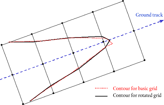
The straightforward way to avoid this effect is to tighten the grid. However this increases computation time. A more elegant solution is to rotate the computation grid so that its direction is parallel to the main ground tracks (i.e. usually parallel to the main runway). Figure 2.7.t shows the effect of such a grid rotation on the contour shape.
2.7.28. Tracing of contours U.K.
A very time-efficient algorithm that eliminates the need to calculate a complete grid array of index values at the expense of a little more computational complexity is to trace the path of the contour, point by point. This option requires two basic steps to be performed and repeated (see Figure 2.7.u):

Step 1 is to find a first point P1 on the contour. This is done by calculating the noise index levels L in equidistant steps along a ‘search ray’ that is expected to cross the required contour of level LC . When the contour is crossed, the difference δ = LC – L changes sign. If this happens, the step-width along the ray is halved and the search direction is reversed. This is done until δ is smaller than a pre-defined accuracy threshold.
Step 2, which is repeated until the contour is sufficiently well defined, is to find the next point on the contour LC — which is at a specified straight line distance r from the current point. During consecutive angular steps, index levels and differences δ are calculated at the ends of vectors describing an arc with radius r. By similarly halving and reversing the increments, this time in the directions of the vector, the next contour point is determined within a predefined accuracy.

Some constraints shall be imposed to guarantee that the contour is estimated with a sufficient degree of accuracy (see Figure 2.7.v):
(1)
The length of the chord Δc (the distance between two contour points) shall be within an interval [Δcmin , Δcmax ], e.g. [10 m, 200 m].
(2)
The length ratio between two adjacent chords of lengths Δcn and Δcn+1 shall be limited, e.g. 0,5 < Δcn /Δcn + 1 < 2.
(3)
With respect to a good fit of the chord length to the contour curvature the following condition shall be fulfilled:
Φn · max(Δcn – 1 , Δcn ) ≤ ε(ε≈ 15 m)
where Φn is the difference in the chord headings.
Experience with this algorithm has shown that, on an average, between 2 and 3 index values have to be calculated to determine a contour point with an accuracy of better than 0,01 dB.
Especially when large contours have to be calculated this algorithm speeds up computation time dramatically. However it should be noted that its implementation requires experience, especially when a contour breaks down into separate islands.
2.8. Assigning noise levels and population to buildings U.K.
For the assessment of the noise exposure of the population only residential buildings shall be considered. No people shall be assigned to other buildings without residential use such as schools, hospitals, office buildings or factories. The assignment of the population to the residential buildings shall be based on the latest official data (depending on the Member State's relevant regulations).
Because aircraft calculation are performed on a 100 m × 100 m resolution grid, the specific case of aircraft noise, levels shall be interpolated based on the nearest grid noise levels.
Determination of the number of inhabitants of a building U.K.
The number of inhabitants of a residential building is an important intermediate parameter for the estimation of the exposure to noise. Unfortunately, data on this parameter is not always available. Below it is specified how this parameter can be derived from data more readily available.
Symbols used in the following are:
BA
=
base area of the building
DFS
=
dwelling floor space
DUFS
=
dwelling unit floor space
H
=
height of the building
FSI
=
dwelling floor space per inhabitant
Inh
=
number of inhabitants
NF
=
number of floors
V
=
volume of residential buildings
For the calculation of the number of inhabitants, either the following case 1 procedure or the case 2 procedure shall be used, depending on the availability of data.
CASE 1: the data on the number of inhabitants is available U.K.
1A
:
The number of inhabitants is known or has been estimated on the basis of dwelling units. In this case the number of inhabitants of a building is the sum of the number of inhabitants of all dwelling units in the building:

1B
:
The number of inhabitants is known only for entities larger than a building, e.g. sides of city blocks, city blocks, districts or even an entire municipality. In this case the number of inhabitants of a building is estimated based on the volume of the building:

The index ‘total’ here refers to the respective entity considered. The volume of the building is the product of its base area and its height:
| Vbuilding = BAbuilding × Hbuilding | (2.8.3) |
If the height of the building is not known, it shall be estimated based on the number of floors NFbuilding , assuming an average height per floor of 3 m:
| Hbuilding = NFbuilding × 3 m | (2.8.4) |
If the number of floors is also not known, a default value for the number of floors representative of the district or the borough shall be used.
The total volume of residential buildings in the entity considered Vtotal is calculated as the sum of the volumes of all residential buildings in the entity:

CASE 2: no data on the number of inhabitants is available U.K.
In this case the number of inhabitants is estimated based on the average dwelling floor space per inhabitant FSI. If this parameter is not known, a national default value shall be used.
2A
:
The dwelling floor space is known on the basis of dwelling units. In this case the number of inhabitants of each dwelling unit is estimated as follows:

The number of inhabitants of the building can now be estimated as in CASE 1A above.
2B
:
The dwelling floor space is known for the entire building, i.e. the sum of the dwelling floor spaces of all dwelling units in the building is known. In this case the number of inhabitants is estimated as follows:

2C
:
The dwelling floor space is known only for entities larger than a building, e.g. sides of city blocks, city blocks, districts or even an entire municipality.
In this case the number of inhabitants of a building is estimated based on the volume of the building as described in CASE 1B above with the total number of inhabitants estimated as follows:

2D
:
The dwelling floor space is unknown. In this case the number of inhabitants of a building is estimated as described in CASE 2B above with the dwelling floor space estimated as follows:
| DFSbuilding = BAbuilding × 0,8 × NFbuilding | (2.8.9) |
The factor 0,8 is the conversion factor gross floor area → dwelling floor space. If a different factor is known to be representative of the area it shall be used instead and clearly documented.
If the number of floors of the building is not known, it shall be estimated based on the height of the building, Hbuilding , typically resulting in a non-integer number of floors:

If neither the height of the building nor the number of floors is known, a default value for the number of floors representative of the district or the borough shall be used.
Assigning receiver points to the façades of buildings U.K.
The assessment of population exposure to noise is based on receiver point levels at 4 m above the terrain level in front of building façades of residential buildings.
For the calculation of the number of inhabitants, either the following case 1 procedure or the case 2 procedure shall be used for land based noise sources. For aircraft noise calculated according to 2.6, all population of a building is associated to the nearest noise calculation point on the grid.
CASE 1 U.K.

(a)
Segments of a length of more than 5 m are split up into regular intervals of the longest possible length, but less than or equal to 5 m. Receiver points are placed in the middle of each regular interval.
(b)
Remaining segments above a length of 2,5 m are represented by one receiver point in the middle of each segment.
(c)
Remaining adjacent segments with a total length of more than 5 m are treated as polyline objects in a manner similar to that described in (a) and (b).
(d)
The number of inhabitants allocated to a receiver point, shall be weighted by the length of the represented façade so that the sum over all receiver points represents the total number of inhabitants.
(e)
Only for buildings with floor sizes that indicate a single dwelling per floor level, the most exposed façade noise level is directly used for the statistics and related to the number of inhabitants.
CASE 2 U.K.

(a)
Façades are considered separately or are split up every 5 m from the start position onwards, with a receiver position placed at the half-way distance of the façade or the 5 m segment
(b)
The remaining section has its receiver point in its mid-point.
(c)
The number of inhabitants allocated to a receiver point, shall be weighted by the length of the represented façade so that the sum over all receiver points represents the total number of inhabitants.
(d)
Only for buildings with floor sizes that indicate a single dwelling per floor level, the most exposed façade noise level is directly used for the statistics and related to the number of inhabitants.
3.INPUT DATAU.K.
Input data to be used as appropriate in association with the methods described above are given in Appendix F to Appendix I.
In cases where input data provided in Appendix F to Appendix I are not applicable or cause deviations from the true value that do not meet the conditions presented under 2.1.2 and 2.6.2, other values can be used, provided that the values used and the methodology used to derive them are sufficiently documented, including demonstrating their suitability. This information shall be made publicly available.
4.MEASUREMENT METHODSU.K.
In cases when, for any reason, measurements are performed, these shall be in accordance with the principles governing long term average measurements stated in ISO 1996-1:2003 and ISO 1996-2:2007 or, for aircraft noise, ISO 20906:2009.
(1)
The absorption of porous road pavements is taken into account in the emission model.
(2)
A network of small obstacles in a plane and at regular intervals constitutes one example of a special configuration.
(3)
Actually beneath the aircraft perpendicular to the wing axis and direction of flight; taken to be vertically below the aircraft when in non-turning (i.e. non-banked) flight.
(4)
Time is accounted for via the aircraft speed.
(5)
Displaced thresholds can be taken into account by defining additional runways.
(6)
Calculated levels at 4 m or higher are sometimes requested. Comparison of measurements at 1,2 m and 10 m and theoretical calculation of ground effects show that variations of the A-weighted sound exposure level are relatively insensitive to receiver height. The variations are in general smaller than one decibel, except if the maximum angle of sound incidence is below 10° and if the A-weighted spectrum at the receiver has its maximum in the range of 200 to 500 Hz. Such low frequency dominated spectra may occur e.g. at long distances for low-bypass ratio engines and for propeller engines with discrete low frequency tones.
(7)
Aircraft flight data recorders provide comprehensive operational data. However this is not readily accessible and is costly to provide; thus its use for noise modelling purposes is normally restricted to special projects and model development studies.
(8)
Usually measured as altitude above MSL (i.e. relative to 1 013 mb) and corrected to airport elevation by the airport monitoring system.
(9)
Usually the axes of the local coordinate are parallel to the axis of the map that contours are drawn on. However it is sometimes useful to choose the x-axis parallel to a runway in order to get symmetrical contours without using a fine computational grid (see Sections 2.7.26 to 2.7.28).
(10)
For non-level ground it is possible for the observer to be above the aircraft in which case, for calculating sound propagation z′ (and the corresponding elevation angle β — see Chapter 4) is put equal to zero.
(11)
How best to implement this is left to the user as this will depend on the way in which turn radii are defined. When the starting point is a sequence of straight or circular legs, a relatively simple option is to insert bank angle transition segments at the start of the turn and at its end in which the aircraft rolls at a constant rate (e.g. expressed in °/m or °/s).
(12)
For this purpose the total length of the ground track should always exceed that of the flight profile. This can be achieved, if necessary, by adding straight segments of suitable length to the last segment of the ground track.
(13)
Defined in this simple way, the total length of the segmented path is slightly less than that of the circular path. However the consequent contour error is negligible if the angular increments are below 30°.
(14)
Even if engine power settings remain constant along a segment, propulsive force and acceleration can change due to variation of air density with height. However, for the purposes of noise modelling these changes are normally negligible.
(15)
This was recommended in the previous edition of ECAC Doc 29 but is still considered provisional pending the acquisition of further corroborative experimental data.
(16)
10dB-down LE may be up to 0,5 dB lower than LE evaluated over a longer duration. However, except at short slant distances where event levels are high, extraneous ambient noise often makes longer measurement intervals impractical and 10-dB down values are the norm. As studies of the effects of noise (used to ‘calibrate’ the noise contours) also tend to rely on 10-dB down values, the ANP tabulations are considered to be entirely appropriate.
(17)
Although the notion of an infinitely long flight path is important to the definition of event sound exposure level LE , it has less relevance in the case of event maximum level Lmax which is governed by the noise emitted by the aircraft when at a particular position at or near its closest point of approach to the observer. For modelling purposes the NPD distance parameter is taken to be the minimum distance between the observer and segment.
(18)
NPD specifications require that the data be based on measurements of steady straight flight, not necessarily level; to create the necessary flight conditions, the test aircraft flight path can be inclined to the horizontal. However, as will be seen, inclined paths lead to computational difficulties and, when using the data for modelling, it is convenient to visualise the source paths as being both straight and level.
(19)
This is known as the duration correction because it makes allowance for the effects of aircraft speed on the duration of the sound event — implementing the simple assumption that, other things being equal, duration, and thus received event sound energy, is inversely proportional to source velocity.
(20)
In the case of non-flat terrain there can be different definitions of elevation angle. Here it is defined by the aircraft height above the observation point and the slant distance — hence neglecting local terrain gradients as well as obstacles on the sound propagation path (see Sections 2.7.6 and 2.7.10). In the event that, due to ground elevation, the receiver point is above the aircraft, elevation angle β is set equal to zero.
(21)
A ‘free-field’ level is that which would be observed if the ground surface were not there.
(22)
The wind and temperature gradients and turbulence depend in part upon the roughness and heat transfer characteristics of the surface.
(23)
For an observer located on the right side to the segment φ would become β + ε (see Section 2.7.19).
(24)
The time periods may differ from these three, depending on the definition of the noise index used.
Options/Help
Print Options
PrintThe Whole Directive
PrintThe Whole Annex
PrintThis Division only
You have chosen to open the Whole Directive
The Whole Directive you have selected contains over 200 provisions and might take some time to download. You may also experience some issues with your browser, such as an alert box that a script is taking a long time to run.
Would you like to continue?
You have chosen to open Schedules only
Y Rhestrau you have selected contains over 200 provisions and might take some time to download. You may also experience some issues with your browser, such as an alert box that a script is taking a long time to run.
Would you like to continue?
Mae deddfwriaeth ar gael mewn fersiynau gwahanol:
Y Diweddaraf sydd Ar Gael (diwygiedig):Y fersiwn ddiweddaraf sydd ar gael o’r ddeddfwriaeth yn cynnwys newidiadau a wnaed gan ddeddfwriaeth ddilynol ac wedi eu gweithredu gan ein tîm golygyddol. Gellir gweld y newidiadau nad ydym wedi eu gweithredu i’r testun eto yn yr ardal ‘Newidiadau i Ddeddfwriaeth’.
Gwreiddiol (Fel y’i mabwysiadwyd gan yr UE): Mae'r wreiddiol version of the legislation as it stood when it was first adopted in the EU. No changes have been applied to the text.
Pwynt Penodol mewn Amser: This becomes available after navigating to view revised legislation as it stood at a certain point in time via Advanced Features > Show Timeline of Changes or via a point in time advanced search.
Gweler y wybodaeth ychwanegol ochr yn ochr â’r cynnwys
Rhychwant ddaearyddol: Indicates the geographical area that this provision applies to. For further information see ‘Frequently Asked Questions’.
Dangos Llinell Amser Newidiadau: See how this legislation has or could change over time. Turning this feature on will show extra navigation options to go to these specific points in time. Return to the latest available version by using the controls above in the What Version box.
Dewisiadau Agor
Dewisiadau gwahanol i agor deddfwriaeth er mwyn gweld rhagor o gynnwys ar y sgrin ar yr un pryd
Rhagor o Adnoddau
Gallwch wneud defnydd o ddogfennau atodol hanfodol a gwybodaeth ar gyfer yr eitem ddeddfwriaeth o’r tab hwn. Yn ddibynnol ar yr eitem ddeddfwriaeth sydd i’w gweld, gallai hyn gynnwys:
- y PDF print gwreiddiol y fel adopted version that was used for the EU Official Journal
- rhestr o newidiadau a wnaed gan a/neu yn effeithio ar yr eitem hon o ddeddfwriaeth
- pob fformat o’r holl ddogfennau cysylltiedig
- slipiau cywiro
- dolenni i ddeddfwriaeth gysylltiedig ac adnoddau gwybodaeth eraill
Llinell Amser Newidiadau
Mae’r llinell amser yma yn dangos y fersiynau gwahanol a gymerwyd o EUR-Lex yn ogystal ag unrhyw fersiynau dilynol a grëwyd ar ôl y diwrnod ymadael o ganlyniad i newidiadau a wnaed gan ddeddfwriaeth y Deyrnas Unedig.
Cymerir dyddiadau fersiynau’r UE o ddyddiadau’r dogfennau ar EUR-Lex ac efallai na fyddant yn cyfateb â’r adeg pan ddaeth y newidiadau i rym ar gyfer y ddogfen.
Ar gyfer unrhyw fersiynau a grëwyd ar ôl y diwrnod ymadael o ganlyniad i newidiadau a wnaed gan ddeddfwriaeth y Deyrnas Unedig, bydd y dyddiad yn cyd-fynd â’r dyddiad cynharaf y daeth y newid (e.e. ychwanegiad, diddymiad neu gyfnewidiad) a weithredwyd i rym. Am ragor o wybodaeth gweler ein canllaw i ddeddfwriaeth ddiwygiedig ar Ddeall Deddfwriaeth.
Rhagor o Adnoddau
Defnyddiwch y ddewislen hon i agor dogfennau hanfodol sy’n cyd-fynd â’r ddeddfwriaeth a gwybodaeth am yr eitem hon o ddeddfwriaeth. Gan ddibynnu ar yr eitem o ddeddfwriaeth sy’n cael ei gweld gall hyn gynnwys:
- y PDF print gwreiddiol y fel adopted fersiwn a ddefnyddiwyd am y copi print
- slipiau cywiro
liciwch ‘Gweld Mwy’ neu ddewis ‘Rhagor o Adnoddau’ am wybodaeth ychwanegol gan gynnwys
- rhestr o newidiadau a wnaed gan a/neu yn effeithio ar yr eitem hon o ddeddfwriaeth
- manylion rhoi grym a newid cyffredinol
- pob fformat o’r holl ddogfennau cysylltiedig
- dolenni i ddeddfwriaeth gysylltiedig ac adnoddau gwybodaeth eraill
 Mae’r holl gynnwys ar gael dan Drwydded Llywodraeth Agored v3.0 ac eithrio ble nodir yn wahanol. Yn ychwanegol mae’r safle hwn â chynnwys sy’n deillio o EUR-Lex, a ailddefnyddiwyd dan delerau Penderfyniad y Comisiwn 2011/833/EU ar ailddefnyddio dogfennau o sefydliadau’r UE. Am ragor o wybodaeth gweler ddatganiad cyhoeddus Swyddfa Gyhoeddiadau’r UE ar ailddefnyddio.