
Appendix E The finite segment correction
This appendix outlines the derivation of the finite segment correction and the associated energy fraction algorithm described in Section 2.7.19.
E1GEOMETRYU.K.
The energy fraction algorithm is based on the sound radiation of a ‘fourth-power’ 90-degree dipole sound source. This has directional characteristics which approximate those of jet aircraft sound, at least in the angular region that most influences sound event levels beneath and to the side of the aircraft flight path.

Figure E-1 illustrates the geometry of sound propagation between the flight path and the observer location O. The aircraft at P is flying in still uniform air with a constant speed on a straight, level flight path. Its closest point of approach to the observer is Pp . The parameters are:
distance from the observer to the aircraft
perpendicular distance from the observer to the flight path (slant distance)
distance from P to Pp = – V · τ
speed of the aircraft
time at which the aircraft is at point P
time at which the aircraft is located at the point of closest approach Pp
flight time = time relative to time at Pp = t – tp
angle between flight path and aircraft-observer vector
It should be noted that, since the flight time τ relative to the point of closest approach is negative when the aircraft is before the observer position (as shown in Figure E-1), the relative distance q to the point of closest approach becomes positive in that case. If the aircraft is ahead of the observer, q becomes negative.
E2ESTIMATION OF THE ENERGY FRACTIONU.K.
The basic concept of the energy fraction is to express the noise exposure E produced at the observer position from a flight path segment P1P2 (with a start-point P1 and an end-point P2 ) by multiplying the exposure E∞ from the whole infinite path flyby by a simple factor — the energy fraction factor F:
| E = F · E∞ | (E-1) |
Since the exposure can be expressed in terms of the time-integral of the mean-square (weighted) sound pressure level, i.e.

to calculate E, the mean-square pressure has to be expressed as a function of the known geometric and operational parameters. For a 90° dipole source,
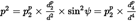
where p 2 and pp 2 are the observed mean-square sound pressures produced by the aircraft as it passes points P and Pp .
This relatively simple relationship has been found to provide a good simulation of jet aircraft noise, even though the real mechanisms involved are extremely complex. The term dp 2/d2 in equation E-3 describes just the mechanism of spherical spreading appropriate to a point source, an infinite sound speed and a uniform, non-dissipative atmosphere. All other physical effects — source directivity, finite sound speed, atmospheric absorption, Doppler-shift etc. — are implicitly covered by the sin2ψ term. This factor causes the mean square pressure to decrease inversely as d4 ; whence the expression ‘fourth power’ source.
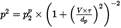
Introducing the substitutions


the mean-square pressure can be expressed as a function of time (again disregarding sound propagation time):
Putting this into equation (E-2) and performing the substitution

the sound exposure at the observer from the flypast between the time interval [τ1 ,τ2 ] can be expressed as

The solution of this integral is:

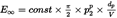
Integration over the interval [–∞,+∞] (i.e. over the whole infinite flight path) yields the following expression for the total exposure E∞ :
and hence the energy fraction according to equation E-1 is

E3CONSISTENCY OF MAXIMUM AND TIME INTEGRATED METRICS — THE SCALED DISTANCEU.K.
A consequence of using the simple dipole model to define the energy fraction is that it implies a specific theoretical difference ΔL between the event noise levels Lmax and LE . If the contour model is to be internally consistent, this needs to equal the difference of the values determined from the NPD curves. A problem is that the NPD data are derived from actual aircraft noise measurements — which do not necessarily accord with the simple theory. The theory therefore needs an added element of flexibility. But in principal the variables α1 and α2 are determined by geometry and aircraft speed — thus leaving no further degrees of freedom. A solution is provided by the concept of a scaled distance dλ as follows.
The exposure level LE,∞ as tabulated as a function of dp in the ANP database for a reference speed Vref, can be expressed as

where p 0 is a standard reference pressure and tref is a reference time (= 1 s for SEL). For the actual speed V it becomes

Similarly the maximum event level Lmax can be written

For the dipole source, using equations E-8, E-11 and E-12, noting that (from equations E-2 and E-8) 

This can only be equated to the value of ΔL determined from the NPD data if the slant distance dp used to calculate the energy fraction is substituted by a scaled distance dλ given by

or
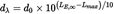

Replacing dp by dλ in equation E-5 and using the definition q = Vτ from Figure E-1 the parameters α1 and α2 in equation E-9 can be written (putting q = q1 at the start-point and q – λ = q2 at the endpoint of a flight path segment of length λ) as


Having to replace the slant actual distance by scaled distance diminishes the simplicity of the fourth-power 90 degree dipole model. But as it is effectively calibrated in situ using data derived from measurements, the energy fraction algorithm can be regarded as semi-empirical rather than a pure theoretical.